YouTube Video Review version:

Information

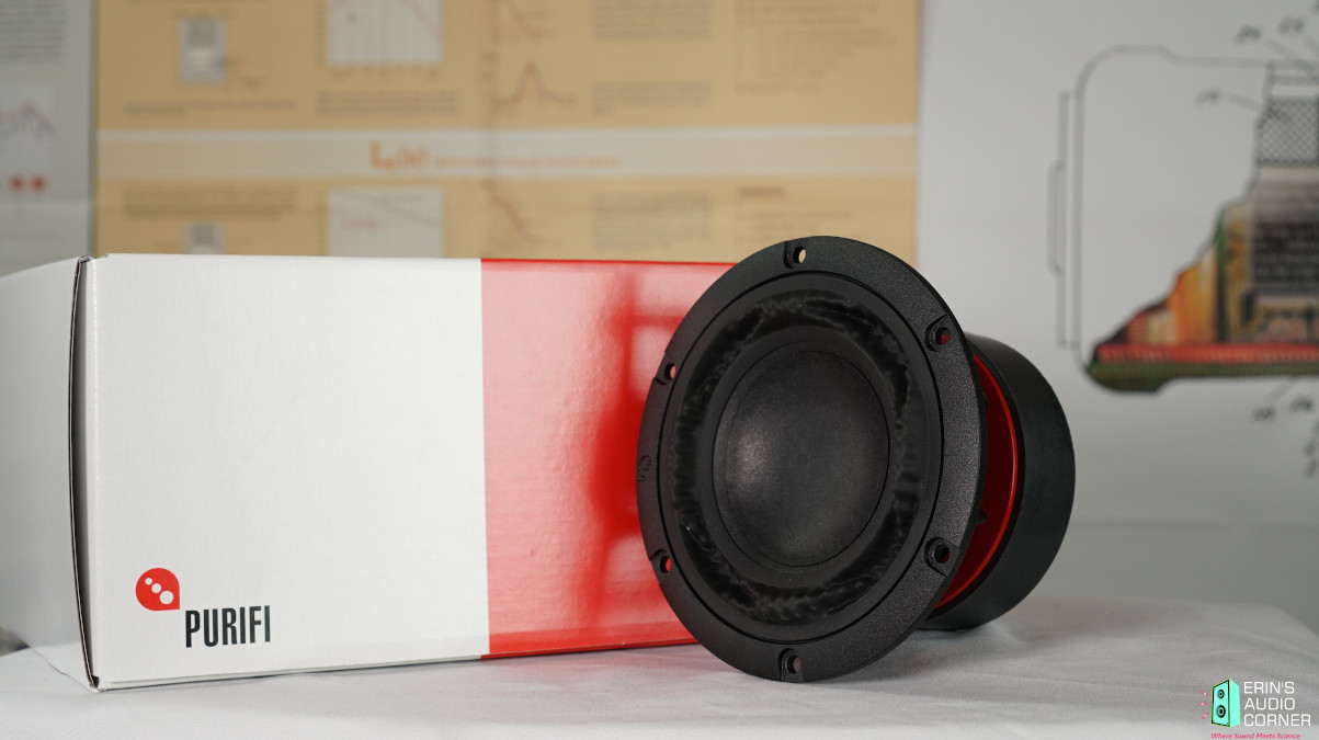
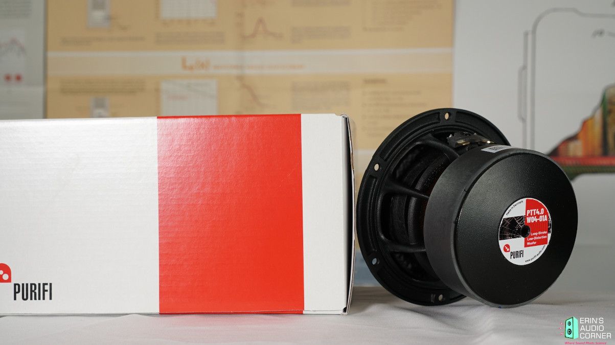
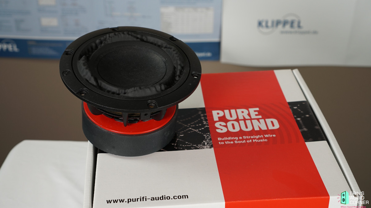
The Purifi Audio PTT4.0W04 is a long linear throw 4-inch midwoofer which costs about $580/pair USD. It has so much science baked in to its design that it makes my mind hurt so rather than try to pretend I understand it all, I’ll just redirect you toward the manufacturer’s website or you can view and purchase them from Madisound if you’d like.

Madisound Enclosure Suggestions:

• .08 -.30 cf sealed for an F3 of 113Hz, F6 of 71Hz, F10 of 45Hz
• .15 cf with a 1” dia. x 5” long port for an F3 of 46Hz
• .25 cf with a 1.5” dia. x 6” long port for an F3 of 43Hz
• .35 cf with a 1.5” dia. x 5.5” long port for an F3 of 39Hz
• .45 cf with a 1.5” dia. x 4.75” long port for an F3 of 36Hz

Test Results

Foreword: Subjective Analysis vs Objective Data of Drive Units (click here)

While I would love to be able to confidently do so, I do not provide subjective analysis of raw drive units. Realistically, there is no easy way or meaningful way to do so. Drive units are parts of a whole. In order to test, subjectively, you would want to integrate it into a system and find what works best when mated to another driver (like a midwoofer to a tweeter, a midrange to a midwoofer, etc.). And to give it a fair shake it must be optimized in that inegration which would be a very arduous task to perform for every drive unit I review. It makes no sense to subjectively critique a single drive unit on its own because it may be used in a different configuration than someone else. One person may cross it with an LR2 HPF and LR4 LPF where another may use it in a completely different bandpass with completely different crossover and slopes. And if I were to try to create a speaker from it for the point of subjective analysis I am left with the same issue. The best implementation for a 6.5-inch midwoofer is different than it is for an 8-inch midwoofer. The data tells the story of performance on an apples-to-apples basis far better than someone's subjective imagination can.

For all the reasons listed above: What I provide here is objective-heavy analysis. However, I provide my own subjective experience and provide insight into what I believe might be positive or negative performance characteristics based on the objective data.

Small Signal Testing (Thiele-Small Results)

Using Klippel’s Distortion Analyzer 2, Linear Lumped Parameter Measurement Module, Pro Driver Stand and provided Panasonic ANR12821 Laser along with Klippel’s Training 1 - Linear Lumped Parameter Measurement tutorial, I measured this drive unit’s impedance and small-signal parameters. Below are the results.

Note: The impedance graph can be found in the Frequency Response Linearity graphic later in this review.

Electrical Parameters
Re	3.71	Ohm	electrical voice coil resistance at DC
Le	0.191	mH	frequency independent part of voice coil inductance
L2	0.396	mH	para-inductance of voice coil
R2	2.10	Ohm	electrical resistance due to eddy current losses
Cmes	369.56	µF	electrical capacitance representing moving mass
Lces	33.15	mH	electrical inductance representing driver compliance
Res	54.22	Ohm	resistance due to mechanical losses
fs	45.5	Hz	driver resonance frequency
Mechanical Parameters
(using laser)
Mms	13.081	g	mechanical mass of driver diaphragm assembly including air load and voice coil
Mmd (Sd)	12.599	g	mechanical mass of voice coil and diaphragm without air load
Rms	0.653	kg/s	mechanical resistance of total-driver losses
Cms	0.937	mm/N	mechanical compliance of driver suspension
Kms	1.07	N/mm	mechanical stiffness of driver suspension
Bl	5.950	N/A	force factor (Bl product)
Lambda s	0.089		suspension creep factor
Loss factors
Qtp	0.367		total Q-factor considering all losses
Qms	5.725		mechanical Q-factor of driver in free air considering Rms only
Qes	0.392		electrical Q-factor of driver in free air considering Re only
Qts	0.367		total Q-factor considering Re and Rms only
Other Parameters
Vas	4.2610	l	equivalent air volume of suspension
n0	0.098	%	reference efficiency (2 pi-radiation using Re)
Lm	82.13	dB	characteristic sound pressure level (SPL at 1m for 1W @ Re)
Lnom	82.45	dB	nominal sensitivity (SPL at 1m for 1W @ Zn)
Sd	56.70	cm²	diaphragm area

Large Signal Modeling (Linear Xmax Results)

Using Klippel’s Distortion Analyzer 2, Large Signal Identification Module, Pro Driver Stand and provided Panasonic ANR12821 Laser along with Klippel’s Training 3 - Loudspeaker Nonlinearities tutorial, I measured the linear, nonlinear and thermal parameters of this drive unit.

Nonlinearities

Traditionally, Xmax has been defined in one of the following ways:

• the physical overhang of the voice coil (height of the voice coil relative to height of the gap)
• 115% times the physical overhang above
• the point where displacement limit(s) is/are exceeded

The third option is where the Klippel LSI module comes in to play. It permits a more “apples to apples” approach of defining the displacement (Xmax) limits based on the XBL, XC, XL and Xd. The displacement limits XBL, XC, XL and Xd describe the limiting effect for the force factor Bl(x), compliance Cms(x), inductance Le(x) and Doppler effect, respectively, according to the threshold values Blmin, Cmin, Zmax and d2 used by the operator.

There are one of two sets of thresholds which can be used to define linear excursion:

1. Non-Subwoofer Drivers: The thresholds Blmin= 82 %, Cmin=75 %, Zmax=10 % and d2=10% generate for a two-tone-signal (f1=fs, f2=8.5fs) 10 % total harmonic distortion and 10 % intermodulation distortion.
2. Subwoofer Drivers: The thresholds Blmin= 70 %, Cmin=50 %, Zmax=17 % create 20 % total harmonic distortion which is becoming the standard for acceptable subwoofer distortion thresholds.

These parameters are defined in more detail in the (Klippel) papers:

• “AN04 – Measurement of Peak Displacement Xmax”
• “AN05 - Displacement Limits due to Driver Nonlinearities”
• “AN17 - Credibility of Nonlinear Parameters”
• “Prediction of Speaker Performance at High Amplitudes”
• “Assessment of Voice Coil Peak Displacement Xmax”
• “Assessing Large Signal Performance of Loudspeakers”

Below are the displacement limits’ results for this drive unit obtained from Klippel’s LSI module:

Displacement Limits
X Bl @ Bl min=82%	>7.6	mm	Displacement limit due to force factor variation
X C @ C min=75%	4.7	mm	Displacement limit due to compliance variation
X L @ Z max=10 %	>7.6	mm	Displacement limit due to inductance variation
X d @ d2=10%	26.8	mm	Displacement limit due to IM distortion (Doppler)
Asymmetry (IEC 62458)
Ak	31.72	%	Stiffness asymmetry Ak(Xpeak)
Xsym	0.12	mm	Symmetry point of Bl(x) at maximal excursion

Per the above table, this drive unit’s linear excursion is limited to 4.7mm due to exceeding the compliance variation displacement limit of 75% for the distortion limit of 10%.

To those who have used KLIPPEL’s LSI module you’ll know why Bl did not resolve. For those wondering why the “greater than” sign shows up for Bl, that’s because the drive unit would have to have been pushed more harder than I deemed necessary to get the data I needed. Possibly, causing damage. Since all I need to know is what the IEC standard xmax value is I stopped once it resolved with Cms.

We can break the above information down further. The below text is written by Patrick Turnmire of Red Rock Acoustics and used with his permission, substituting data from this drive unit’s test results where applicable.

Large Signal Modeling

At higher amplitudes, loudspeakers produce substantial distortion in the output signal, generated by nonlinear ties inherent in the transducer. The dominant nonlinear distortions are predictable and are closely related with the general principle, particular design, material properties and assembling techniques of the loudspeaker. The Klippel Distortion Analyzer combines nonlinear measurement techniques with computer simulation to explain the generation of the nonlinear distortions, to identify their physical causes and to give suggestion for constructional improvements. Better insight into the nonlinear mechanisms makes it possible to further optimize the transducer in respect with sound quality, weight, size and cost.

Nonlinear Characteristics

The dominant nonlinearities are modelled by variable parameters such as

Bl(x)	instantaneous electro-dynamic coupling factor (force factor of the motor) defined by the integral of the magnetic flux density B over voice coil length l as a function of displacement
KMS(x)	mechanical stiffness of driver suspension a function of displacement
LE(i)	voice coil inductance as a function of input current (describes nonlinear permeability of the iron path)
LE(x)	voice coil inductance as a function of displacement

Nonlinear Parameters

Bl change with excursion

The electrodynamic coupling factor, also called Bl-product or force factor Bl(x), is defined by the integral of the magnetic flux density B over voice coil length l and translates current into force. In traditional modeling this parameter is assumed to be constant. The force factor Bl(0) at the rest position corresponds with the Bl-product used in linear modeling. The red curve displays Bl over the entire displacement range covered during the measurement. You see the typical decay of Bl when the voice coil moves out of the gap. At the end of the measurement, the black curve shows the confidential range (interval where the voice coil displacement in this range occurred 99% of the measurement time). During the measurement, the black curve shows the current working range. The dashed curve displays Bl(x) mirrored at the rest position of the voice coil – this way, asymmetries can be quickly identified. Since a laser was connected during the measurement, a coil in / coil out marker is displayed on the bottom left / bottom right.

Suspension Stiffness change with excursion

The stiffness KMS(x) describes the mechanical properties of the suspension. Its inverse is the compliance CMS(x).

Inductance change with excursion

The inductance components Le (x) and Bl(i) of most drivers have a strong asymmetric characteristic. If the voice coil moves towards the back plate the inductance usually increases since the magnetic field generated by the current in the voice coil has a lower magnetic resistance due to the shorter air path. The nonlinear inductance Le(x) has two nonlinear effects. First the variation of the electrical impedance with voice coil displacement x affects the input current of the driver. Here the nonlinear source of distortion is the multiplication of displacement and current. The second effect is the generation of a reluctance force which may be interpreted as an electromagnetic motor force proportional to the squared input current.

The flux modulation Bl(i) has two effects too. On the electrical side the back EMF Bl(i)*v produces nonlinear distortion due to the multiplication of current i and velocity v. On the mechanical side the driving force F = Bl(i)*i comprises a nonlinear term due to the squared current i. This force produces similar effects as the variable term Le(x).

Fs shift with excursion

Qts change with excursion

Asymmetrical Nonlinearities

Asymmetrical nonlinearities produce not only second- and higher-order distortions but also a dc-part in the displacement by rectifying low frequency components. For an asymmetric stiffness characteristic the dc-components moves the voice coil for any excitation signal in the direction of the stiffness minimum. For an asymmetric force factor characteristic the dc-component depends on the frequency of the excitation signal. A sinusoidal tone below resonance (f<fS) would generate or force moving the voice coil always in the force factor maximum. This effect is most welcome for stabilizing voice coil position. However, above the resonance frequency (f>fS) would generate a dc-component moving the voice coil in the force factor minimum and may cause severe stability problems. For an asymmetric inductance characteristic the dc-component moves the voice coil for any excitation signal in the direction of the inductance maximum. Please note that the dynamically generated DC-components cause interactions between the driver nonlinearities. An optimal rest position of the coil in the gap may be destroyed by an asymmetric compliance or inductance characteristic at higher amplitudes. The module Large Signal Simulation (SIM) allows systematic investigation of the complicated behavior.

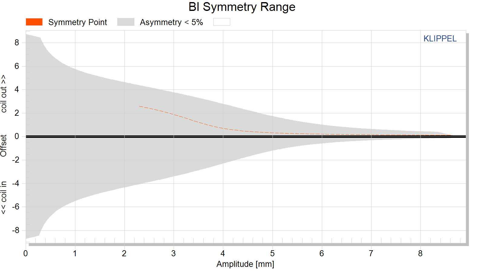
Bl symmetry xb(x)

This curve shows the symmetry point in the nonlinear Bl-curve where a negative and positive displacement x=xpeak will produce the same force factor Bl(xb(x) + x) = Bl(xb(x) – x).

If the shift xb(x) is independent on the displacement amplitude x then the force factor asymmetry is caused by an offset of the voice coil position and can be simply compensated.

If the optimal shift xb(x) varies with the displacement amplitude x then the force factor asymmetry is caused by an asymmetrical geometry of the magnetic field and cannot completely be compensated by coil shifting.

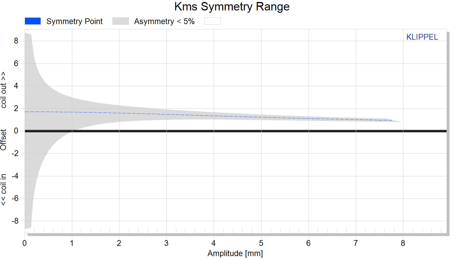
Kms Symmetry xc(x)

This curve shows the symmetry point in the nonlinear compliance curve where a negative and positive displacement x=xpeak will produce the same compliance value kms(xc(x) + x) = kms(xc(x) – x).

A high value of the symmetry point xc(x) at small displacement amplitudes x » 0 indicates that the rest position does not agree with the minimum of the stiffness characteristic. This may be caused by an asymmetry in the geometry of the spider (cup form) or surround (half wave). A high value of the symmetry point xc(x) at maximal displacement x» xmax may be caused by asymmetric limiting of the surround.

Parameters at the Rest Position

For accurate system modelling “Large + Cold” parameters are preferable to “Small Signal” parameters because they more closely reflect the parameters in their typical operating range.

Symbol	Large + Warm	Large + Cold	Small Signal	Unit	Comment
Note:					for accurate small signal parameters, use LPM module
———————–	——–	——–	——–	——	————————————————————————————————————–
Delta Tv [referenced]	35.5		0	K	increase of voice coil temperature during the measurement referenced to imported Re(Delta Tv=0K)
Delta Tv = Tv-Ta	19.9	0	0	K	increase of voice coil temperature during the measurement
Xprot	8.7	8.7	3.0	mm	maximal voice coil excursion (limited by protection system)
Re (Tv)	4.21	3.92	3.92	Ohm	voice coil resistance considering increase of voice coil temperature Tv
Le (X=0)	0.22	0.22	0.22	mH	voice coil inductance at the rest position of the voice coil
L2 (X=0)	0.55	0.55	0.38	mH	para-inductance at the rest position due to the effect of eddy current
R2 (X=0)	0.83	0.83	0.95	Ohm	resistance at the rest position due to eddy currents
Cmes (X=0)	383	383	384	µF	electrical capacitance representing moving mass
Lces (X=0)	58.03	58.03	44.54	mH	electrical inductance at the rest position representing driver compliance
Res (X=0)	56.12	56.12	28.27	Ohm	resistance at the rest position due to mechanical losses
Qms (X=0, Tv)	4.56	4.56	2.62		mechanical Q-factor considering the mechanical system only
Qes (Tv)	0.32	0.30	0.36		electrical Q-factor considering Re (Tv) only
Qts (X=0, Tv)	0.30	0.28	0.32		total Q-factor considering Re (Tv) and Rms only
fs	33.8	33.8	38.5	Hz	driver resonance frequency
Mms	12.596	12.596		g	(calculated from imported Bl) mechanical mass of driver diaphragm assembly including voice-coil and air load
Rms (X=0)	0.587	0.587	1.252	kg/s	mechanical resistance of total-driver losses
Cms (X=0)	1.76	1.76	1.26	mm/N	mechanical compliance of driver suspension at the rest position
Kms (X=0)	0.57	0.57	0.79	N/mm	mechanical stiffness of driver suspension at the rest position
Bl (X=0)	5.95	5.95	5.95	N/A	(imported) force factor at the rest position (Bl product)
Vas	7.9926	7.9926	5.7044	l	equivalent air volume of suspension
N0	0.093	0.100	0.086	%	reference efficiency (2Pi-sr radiation using Re)
Lm	81.8	82.1	81.5	dB	characteristic sound pressure level
Sd	56.70	56.70	56.70	cm²	diaphragm area

Frequency Response

Frequency Response data is generated using Klippel’s Transfer Function Mueasurement module in conjunction with Klippel’s In-Situ Compensation module. This pairing enables me to generate anechoic-quality measurements in the farfield with a resolution of response down to 20Hz increments; far better than splicing nearfield with gated farfield data (the latter of which is often limited to 200Hz or 300Hz resolution and will not show high-Q resonance in the midrange and bass frequencies). Data is represented at 2.83v/1m.

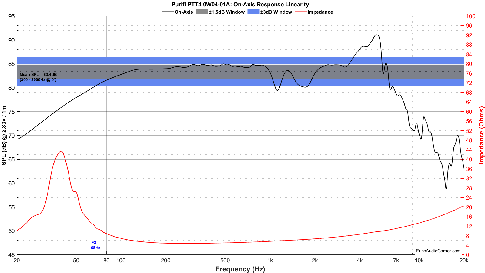
On-Axis Linearity and Impedance

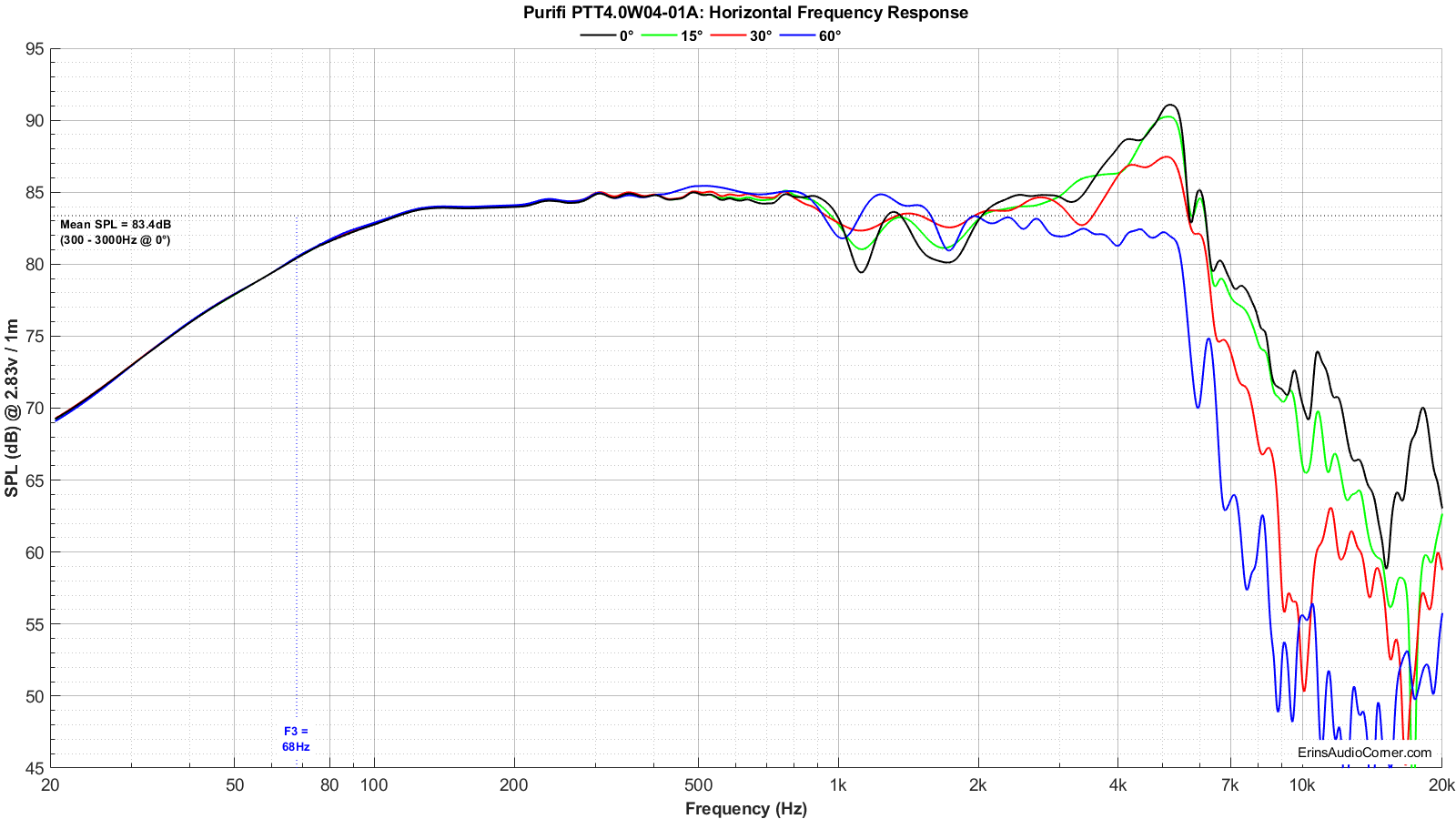
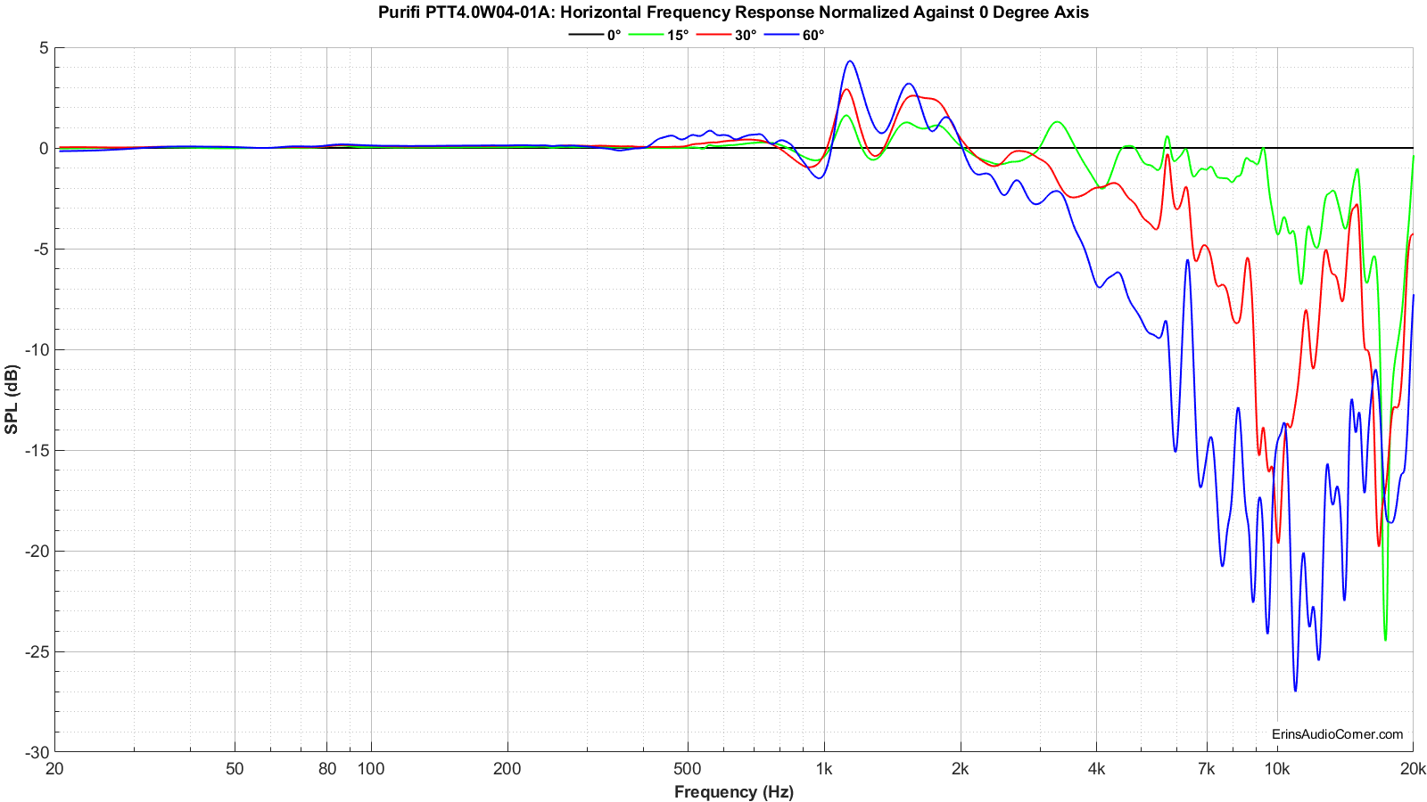
On and Off-Axis Frequency Response

Harmonic Distortion:

Measurements were completed in the nearfield (approximately 0.30 meters with room correction applied via Klippel’s ISC module) using Klippel’s TRF module. Multiple output levels were tested to provide the trend of distortion component profiles and to provide a comparison against other drive units I have tested. The SPL provided is relative to 1 meter distance, averaged in the noted bandpass region.

Intermodulated Distortion (IMD):

Klippel’s 3D-DISTORTION MEASUREMENT (DIS) module is used to calculate the Intermodulated Distortion for this drive unit.

Measurements were completed in the nearfield. Multiple output levels were tested to provide the trend of distortion component profiles and to provide a comparison against other drive units I have tested. The SPL provided is relative to 1 meter distance, averaged in the noted bandpass region.

Unlike Harmonic Distortion - which is a measure of only harmonics from a single tone - IMD is tested with two tones at the same time: a low frequency “bass tone” near Fs and a higher frequency “voice tone” much greater than Fs. For example a speaker driver plays 30Hz at the same time it plays 200Hz. Any distortion artifacts created by the sum and/or difference of the speaker playing both tones at the same time is a result of IMD. In this example, the speaker is supposed to play only 30Hz & 200Hz at the same time. Thanks to IMD, it plays 200Hz ± 30Hz. Second order IMD would be 200 ± 30Hz = 170Hz & 230Hz. Third order IMD would be 200 ± 60Hz = 140Hz & 260Hz. If these ‘side bands’ are high enough in output then they are heard as distortion. If not, they are not.

With that in mind, I used Klippel’s DIS module to test this drive unit in two ways:

1. “Bass tone” fixed at the driver’s Fs, with a “voice sweep” where the 200Hz - 6kHz region is played, one tone at a time (over 50 individual tones).
2. The same as above, but the “bass tone” fixed at 80Hz.

The purpose of me testing with two methods (different “bass tones”) is to see the difference between what happens when the driver plays with high(er) excursion vs when a typical HPF is used. All similarly sized and similarly purposed speakers are tested in the same manner. For better or worse. This means a 6-inch midwoofer is tested the same way an 8-inch midwoofer is. Ultimately, this is for my sanity, because having numerous measurement methods for all sizes of speakers would muddy the waters quickly and wouldn’t give us an idea of when performance is great (say, a 6-inch midwoofer that has much less distortion than an 8-inch) or vice-versa.

The above is tested at 3 voltages each. The first voltage is always 2.83v. The other two voltages are increased to provide higher output (usually targeting at least 96dB for one). As is the case with the multiple HD tests, the multiple IMD levels provides an idea of what the speaker’s IMD profiles look like as the output of the speaker is increased.

Results are provided in GIF form to help understand how the increased output levels impact the distortion profiles and levels. Also, I have provided the (calculated) excursion at the provided tests’ output level so you can see how much excursion the speaker is under at the bass tone. Naturally, with a lower frequency there is higher excursion than with a higher frequency bass tone. This also helps when you are comparing performance against another drive-unit because different speakers have different response profiles; one drive unit may have 2x the excursion from 30Hz to 80Hz while another may have 3x the excursion. Just something to keep in mind.

Test 1: Bass Tone at Fs, Voice Tones from 200-6000Hz

Test 2: Bass Tone at 80Hz, Voice Tones from 200-6000Hz

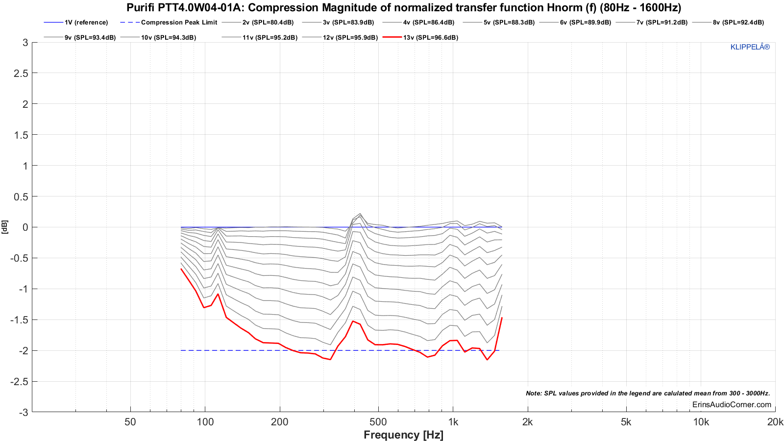
Maximum Long Term SPL (Multitone Distortion Testing) & Compression

Klippel’s Multi-Tone Measurement (MTON) module is used to calculate the maximum SPL for this drive unit.

Unlike IMD testing, Multitone testing incorporates a complex stimulus, used to emulate actual music. However, it is a bit more limited in evaluation purposes so I am using it here to characterize the maximum SPL of a drive unit at 1 meter distance as well as provide how much compression it exhibits with an increase in voice coil temperature.

The below data provides the metrics for how Maximum Long Term SPL is determined. This measurement follows the IEC 60268-21 Long Term SPL protocol, per Klippel’s template, as such:

• Rated maximum sound pressure according IEC 60268-21 §18.4
• Using broadband multi-tone stimulus according §8.4
• Stimulus time = 60 s Excitation time + Preloops according §18.4.1

Each voltage test is 1 minute long (hence, the “Long Term” nomenclature).

The thresholds to determine the maximum SPL are:

• -30dB Distortion relative to the fundamental
• -2dB Compression relative to the reference (1V) measurement

When the speaker has reached either or both above thresholds, the test is terminated and the SPL of the last test is the maximum SPL. In the below results, the legend indicates the average SPL within the same passband as is provided for the Frequency Response measurements. The highest SPL in the legend is the maximum SPL referencd to 1 meter distance. I provide the data showing which threshold was exceeded. The graphic(s) with a red line indicate the threshold that failed and capped the maximum SPL.

This measurement is conducted twice (with a 30-minute break between to let the voice coil cool down):

1. “Midwoofer” - 80Hz to 1600Hz
2. “Midrange” - 200Hz to 4000Hz

The purpose of me testing with two methods is to see how a driver performs in a more “typical” passband vs when it plays an “extended” passband. All similarly sized and similarly purposed speakers are tested in the same manner. For better or worse. This means a 6-inch midwoofer is tested the same way an 8-inch midwoofer is. Ultimately, this is for my sanity, because having numerous measurement methods for all sizes of speakers would muddy the waters quickly and wouldn’t give us an idea of when performance is great (say, a 6-inch midwoofer that has much less distortion than an 8-inch) or vice-versa.

You can watch a demonstration of this testing via my YouTube channel: https://youtu.be/iCjJufvW0IA

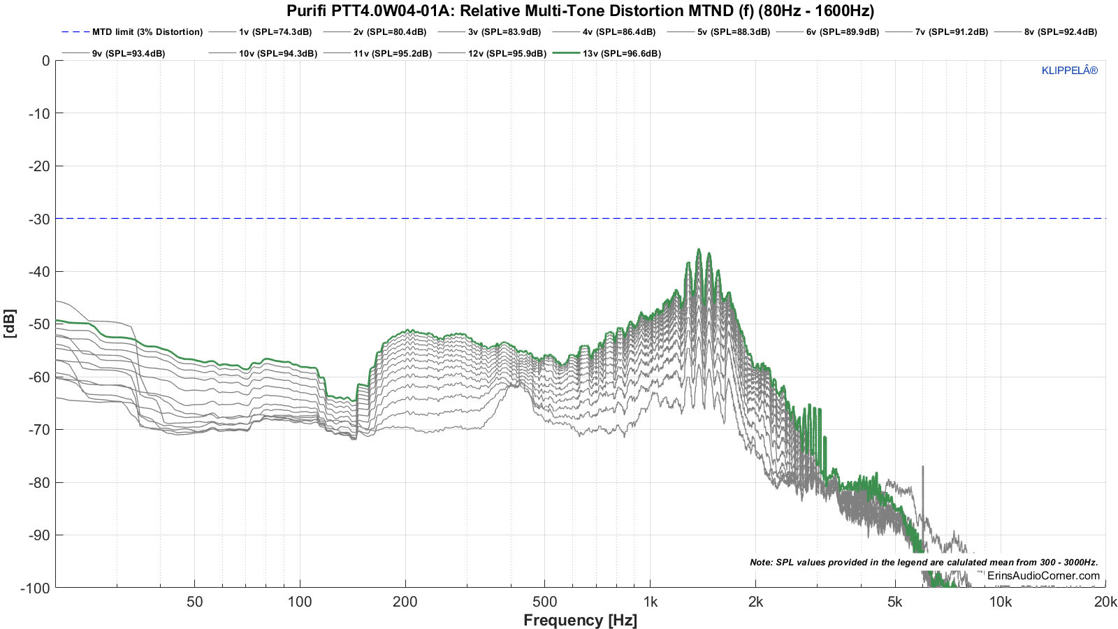
Test 1: Midwoofer

Multitone compression results.

Multitone distortion results.

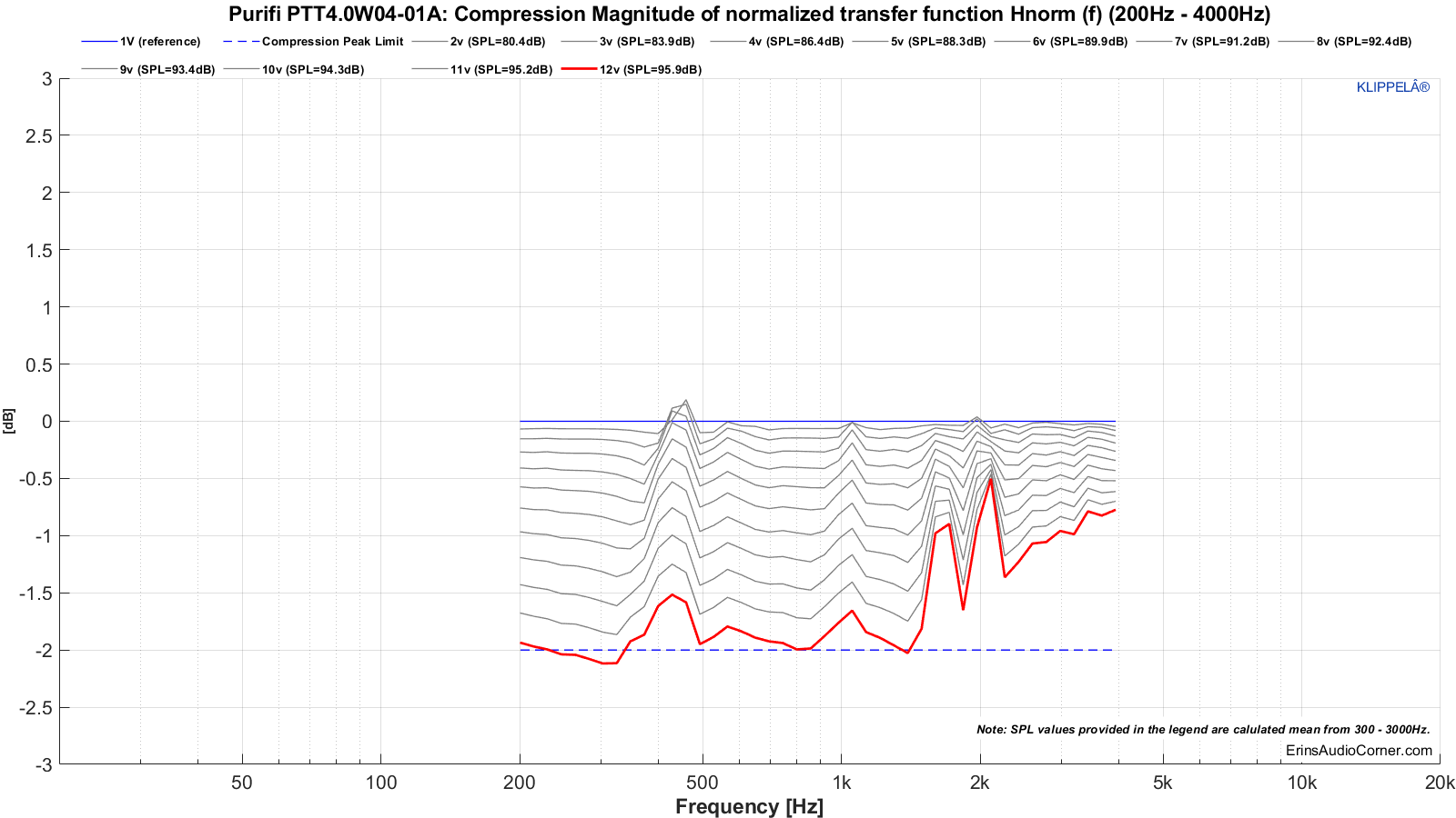
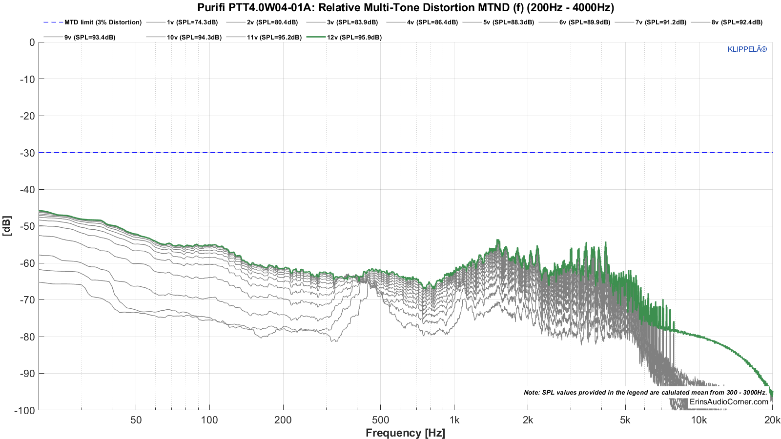
Test 2: Midrange

Multitone compression results.

Multitone distortion results.

The maximum SPL referenced to 1 meter for each test are:

• Max SPL for Test 1 is 96.6dB. The compression threshold was exceeded above this SPL in the midrange above 300Hz.
• Max SPL for Test 1 is 95.9dB. The compression threshold was exceeded above this SPL in the midrange above 300Hz. Same as above. The difference is trivial between the two sets.

Does this mean the speaker will not play above this level? No. It simply means, within a set of limits, the above values are the maximum the speaker output is. Above that SPL, the limits are further and further exceeded.

Bottom Line

Before I get to the test data I want to state this:
This speaker was a bit of an odd bird in regards to how I needed to test its distortion characteristics. It’s not a typical 6 or 7-inch midwoofer and it’s not a typical 4-inch midrange. The designs more fit for this speaker are compact 2-way designs. The low sensitivity makes it not as enticing for midrange in a 3-way. So, I tested it a few ways different than the norm just to get a good idea of how it performs at various tasks. Just keep this in mind if you try to directly compare to other drive units (especially in the same size; they surely won’t perform as well in the midrange distortion facet).

T/S Parameters and Linear Excursion:

• One-way linear excursion measured approximately 4.7mm for this test sample. This is very high for a drive unit this size. I believe this is the longest linear throw from a 4-inch available. But, as you have seen, the price paid is in sensitivity.

Frequency Response:

• The average sensitivity is rather low, measured at about 83.4dB from 300Hz to 3000Hz.
• On-axis response linearity is ±1.5dB within 80-3k Hz if ignoring the 1-2kHz peak/dip I measured.
• On-axis response linearity is ±3.0dB within 68-3.7k Hz if ignoring the 1-2kHz peak/dip I measured.
• Breakup is kept in check to a respectable +7dB at ~5kHz.
• Off-axis response shows nice linearity until about 4kHz.

Distortion and Compression:

• Note: due to the lower sensitivity I was only able to max the HD testing out at about 95dB.
• Distortion at 95dB is: less than 1% THD above 100Hz and greater than 3% THD below 70Hz. Extremely low midrange-distortion profile.

As I said, this Purifi 4-inch midrange drive unit is a bit of an outlier in the world of 4-inch mids. Comparing it to other 4-inch midrange drive units is not a real apples-to-apples given the long excursion/low sensitivity tradeoff this makes in lieu of the typical low excursion/high(ish) sensitivity of typical 4-inch midranges. It may be better suited in comparison to a 5-inch midwoofer. In that regard, I see the advantage for this Purifi 4-inch midrange as being suited for a very compact 2-way system. I’ll be curious to see what DIY designs use this drive unit.

Contribute

If you like what you see here and want to help me keep it going, please consider donating via the PayPal Contribute button at the bottom of each page. Any amount you can chip in to the cause would go a long way toward me keeping the grease on the cogs, paying for server space, hardware, shipping costs, etc. It would be greatly appreciated.

You can also join my Facebook Group and YouTube pages if you’d like to follow along with updates.