Buchardt Audio S400 Bookshelf Speaker Review

YouTube Video Review version:

Intro:

A few months ago, I came across a forum post that touched on Buchardt Audio’s S400 bookshelf speaker. I took a visit to their website to read about it and was (pleasantly) surprised to find the manufacturer provides a set of objective data as well as thorough explanation regarding the design choices. For example: the discussion regarding the tweeter/waveguide assembly and the benefit of controlled directivity (which is, essentially, maintaining the same response profile as the listener moves off-axis from the intended listening axis; the output decreases but the shape varies little when compared to conventional tweeter designs). I don’t have the funds to make costly purchases for review, so I reached out to Mads at Buchardt and inquired about getting a demo pair to try out. Yes, I know to some that is bothersome as it could imply bias but that’s how it is when you’re on a budget and no owner is willing to offer their own samples for test. Mads appreciated that my review goal was objective-data oriented and arranged for me to receive a demo set.

Foreword: Subjective Analysis vs Objective Data (click for more)

If you have seen my past reviews, you know that I am of the mindset that objective data is at least as important as someone's subjective evaluation of a speaker. If not more. Why? Because every room is different. Every listener is different. Some know what to listen for. Others know what they want to hear based on their own preference (i.e., some prefer extended bass, some prefer more midbass punch between 120-150Hz, some prefer a response with a dip around 4kHz, etc., etc.). What one person wants or expects may be opposite of another. Additionally, the room will impact the performance and therefore what the listener hears. This means when you read another's subjective-only review you are left to resolve those variables on your own. That's not likely to happen. Unless there is objective data you can use to get an idea of the performance. With objective data you can begin to understand why the subjective review turned out the way it did. Notably, objective data keeps reviewers honest. It's hard for a reviewer to legitimately bash one product but elevate another when the two measure practically the same in every regard. Not to say two similarly measuring speakers cannot subjectively sound different. Though, odds are if they do measure the same then a huge subjective difference is most likely attributed to other issues such as setup conditions, bias, etc. Objective data is the key to accountability. Simply put: if the measurements are taken with care and you understand them, you can rely on data to help paint a more accurate description of performance than a few adjectives from your favorite reviewer (myself included). As you will see, objective measurements can provide a lot of insight in to how the speaker will perform in your room.

However, when possible, it is always best to demo speakers in your own room. Not simply because of subjective performance. But because of other factors such as aesthetics, pride of ownership, etc. In my experience, all these factors play in to how the listener “connects” with the system. A good shop or manufacturer understands this and allows buyers to try items out at home before purchasing or they offer a reasonable return policy. If you question the performance and can demo the speakers in your own home I suggest you take advantage of the opportunity.

For all the reasons listed above: What I provide here is objective-heavy analysis. I still provide my own subjective experience but with in-room measurements at my listening position(s) so we can understand why I heard what I heard. Is it the room, the actual speaker itself, my brain, or a combination?

Now that you understand my motives, let’s get started with the review.

Product Specs and Photos

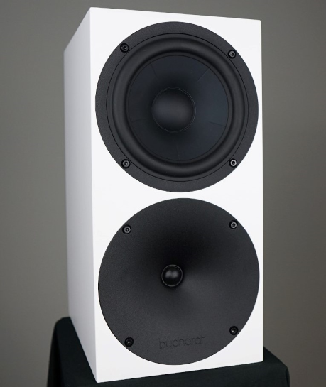
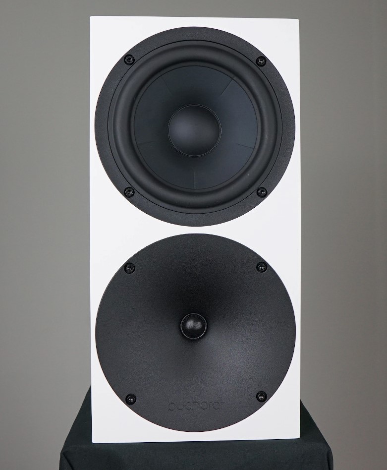
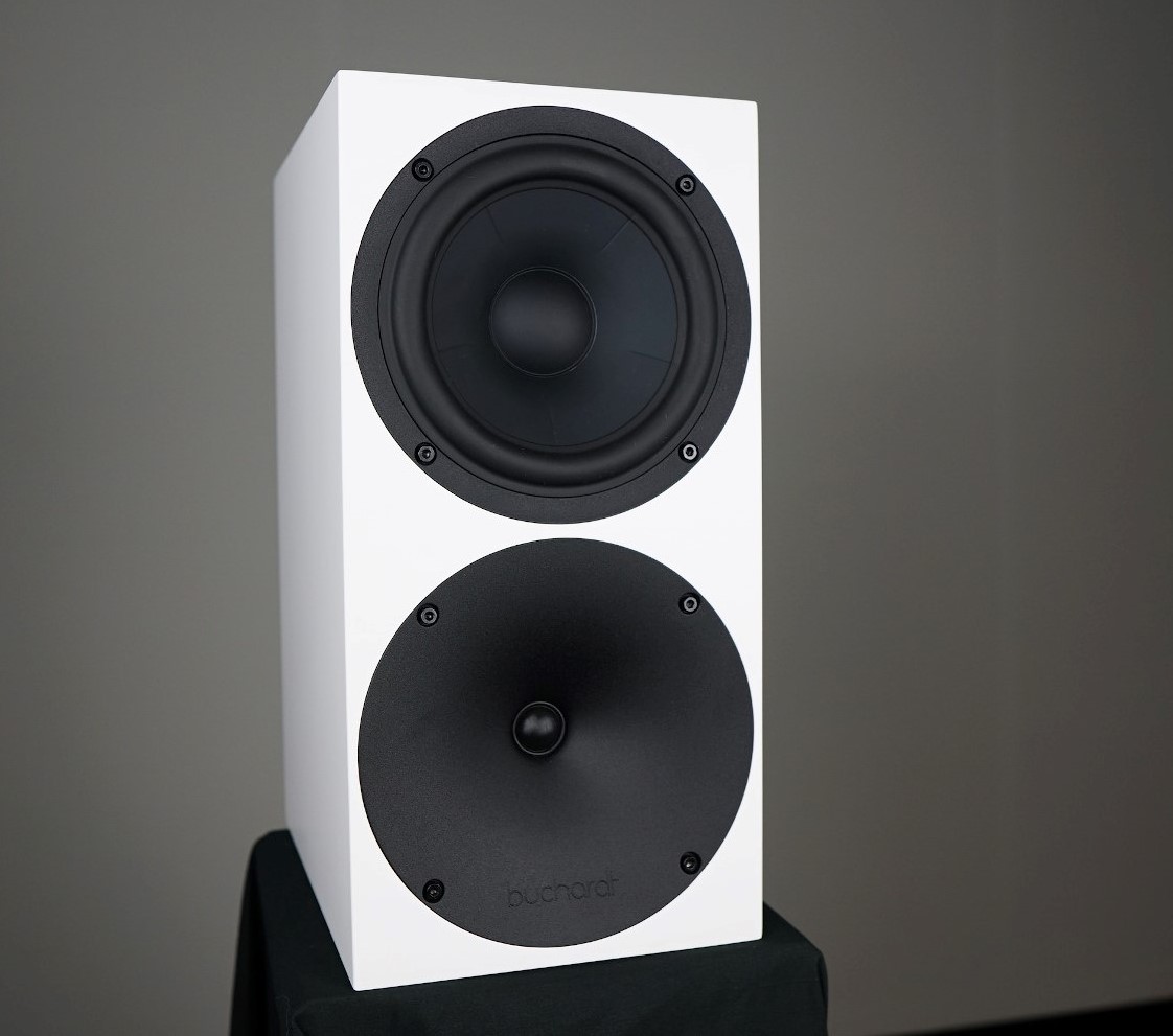
I received this demo pair after a fellow reviewer had his crack and made his YouTube video. Therefore, as expected, there were some blemishes here and there from previous use. No big deal. One thing I like, aesthetically speaking, is the color. I like the stark contrast of the white cabinet vs black speakers. To my eye they just pop. Buchardt does offer other color options as well for those who are not fond of this particular colorway, however. The speaker itself is quite slim at approximately 7 inches wide. The S400 houses a small ~19mm dome tweeter in a rather large waveguide, a 6-inch aluminum cone mid/woofer and a 5x8-inch passive radiator. All drive units are made by SB Acoustics, if you’re wondering. Generally speaking, I like SB Acoustics’ drive units (especially the Satori lineup) and their use here hints at a quality speaker. I don’t know if Buchardt has their own custom drive units manufactured by SB Acoustics for this speaker - I assume they do - but you can find their SB Acoustics counterparts sold by Madisound in the USA. And, yes, the cone of the mid/woofer is the same as what you’ve seen in Harman’s Revel speakers.

The speakers do come with a black grille for both the mid/woofer and tweeter which both magnetically snap in place. However, I prefer the look of these speakers without the grilles. And, as you’ll see later, the performance is better without the grilles.

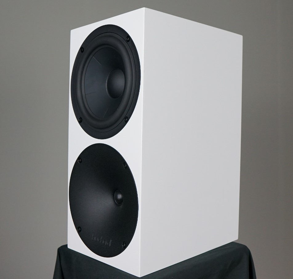
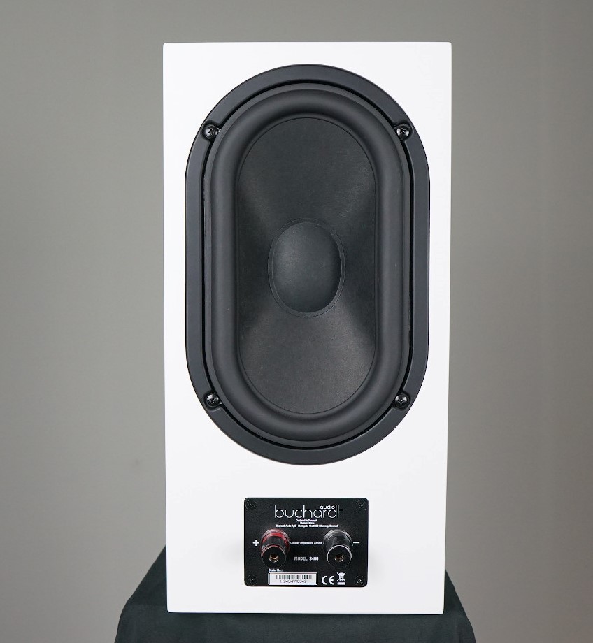
Note the 2° backward slope; an attempt to acoustically align the tweeter with the mid/woofer.

Objective Data

Unless otherwise noted, all the data below was captured using Klippel Distortion Analyzer 2 and Klippel modules (TRF, DIS, LPM, ISC to name a few). Most of the data was exported to a text file and then graphed using my own MATLAB scripts in order to present the data in a specific way I prefer. However, some is given using Klippel’s graphing.

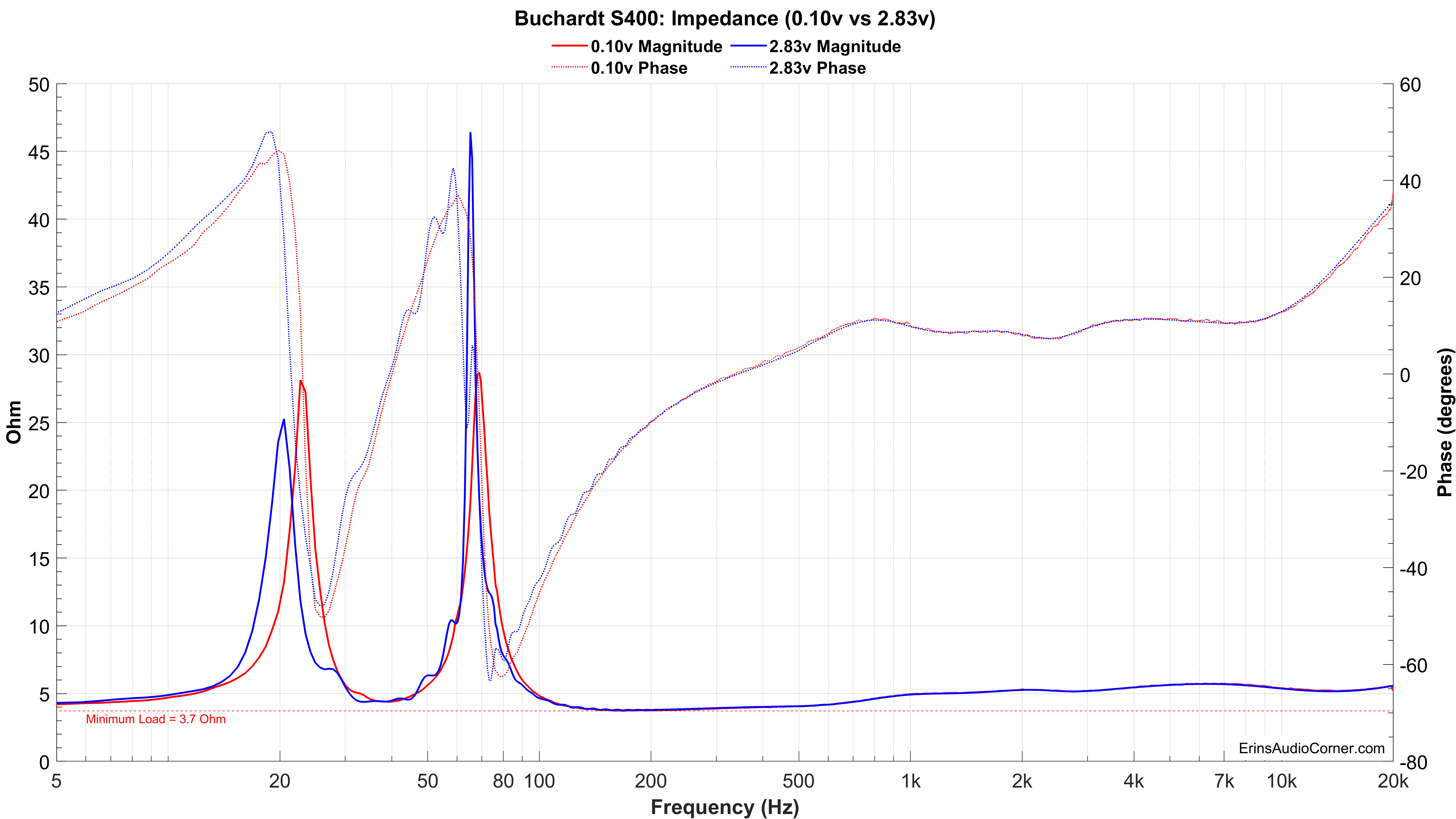
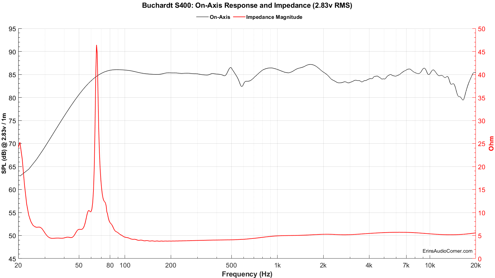
Impedance Phase and Magnitude:

Impedance measurements are provided both at 0.10 volts RMS and 2.83 volts RMS. The low-level voltage version is standard because it ensures the speaker/driver is in linear operating range. The higher voltage is to see what happens when the output voltage is increased to the 2.83vRMS speaker sensitivity test.

Frequency Response:

Notes about measurements (click for info)

Frequency response data (horizontal, vertical, “Spinorama”, polar, spectrograms, etc.) are all based on a 2.83 volts RMS logarithmic sweep at 1 meter to meet the standard sensitivity measurement spec. The measurement axis was between the tweeter and mid/woofer, per the manufacturer’s recommendation. These data are captured using Klippel’s TRF module and a mixture of ground-plane measurement and 4-pi free-field measurement. Klippel’s In-Situ Room Compensation (ISC) module is then used with the ground plane measurement to provide a ‘reference’ curve to the 4-pi measurement which then corrects for the room’s influence and allows me to generate a reflection-free far-field response from an indoors measurement. Note: This is not a standard merge of nearfield and farfield nor a merge of ground-plane and farfield. Typical merged responses still suffer low resolution in the midrange where the response is merged due to the necessity of windowing the impulse response to remove reflections. One major downside to “gating” or “windowing” the impulse response is this low-resolution does not show resonance in the midrange. For example, most free-field measurements are only reflection-free until approximately 3 milliseconds, or about 300Hz. That means a data point every 300Hz. If you have a high-Q resonance at 450Hz the 300Hz resolution data will not show this resonance because the frequency resolution only has a data point at 300Hz and 600Hz; skipping right over the 450Hz. You would need a resolution of at least a half the width of the Q-factor; generally, 20Hz is adequate. However, 20Hz resolution is roughly 50ms of window-free response. The only way to achieve this is in a large parking lot or open field. Ground plane measurements are perfect for this but are subject to aiming/ground absorption (grass) and related issues above 400Hz. The ISC module permits results with as-close-to-anechoic as one can achieve without being anechoic. Thanks to the ISC module, the data I am providing here is higher resolution (~30Hz resolution) than an average person can provide without access to an anechoic chamber or the like.

The measurement below provides the frequency response at the reference measurement axis - also known as the 0-degree axis or “on axis” plane - in this measurement condition was situated between the woofer and waveguide, per the manufacturer recommendation.

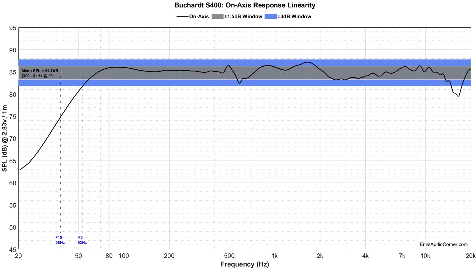
The mean spl, approximately 84.7dB, is calculated over the frequency range of 300Hz to 3,000Hz. The blue shaded area represents the ±3dB response window from this mean spl value. As you can see in the blue window above, the Buchardt S400 has a ±3dB response from 53Hz - ~16kHz, with the latter being a function of the on-axis dip via cancelation of the dome tweeter to the waveguide mouth which is not apparent off-axis. A tighter window of linearity is provided in gray as ±1.5dB from the mean SPL.

The speaker’s F3 point (the frequency at which the response has fallen 3dB relative to the mean spl) is 53Hz and the F10 (the frequency at which the response has fallen by 10dB relative to the mean spl) is 38Hz. While typical rooms provide a low-frequency boost, if you plan to listen to music with lower frequency content, this information indicates you would need a subwoofer to fill in the lower octaves (or, you can use EQ to boost the low end but lowering the maximum SPL). For further discussion on maximum SPL please read by evaluation sections toward the end of this review.

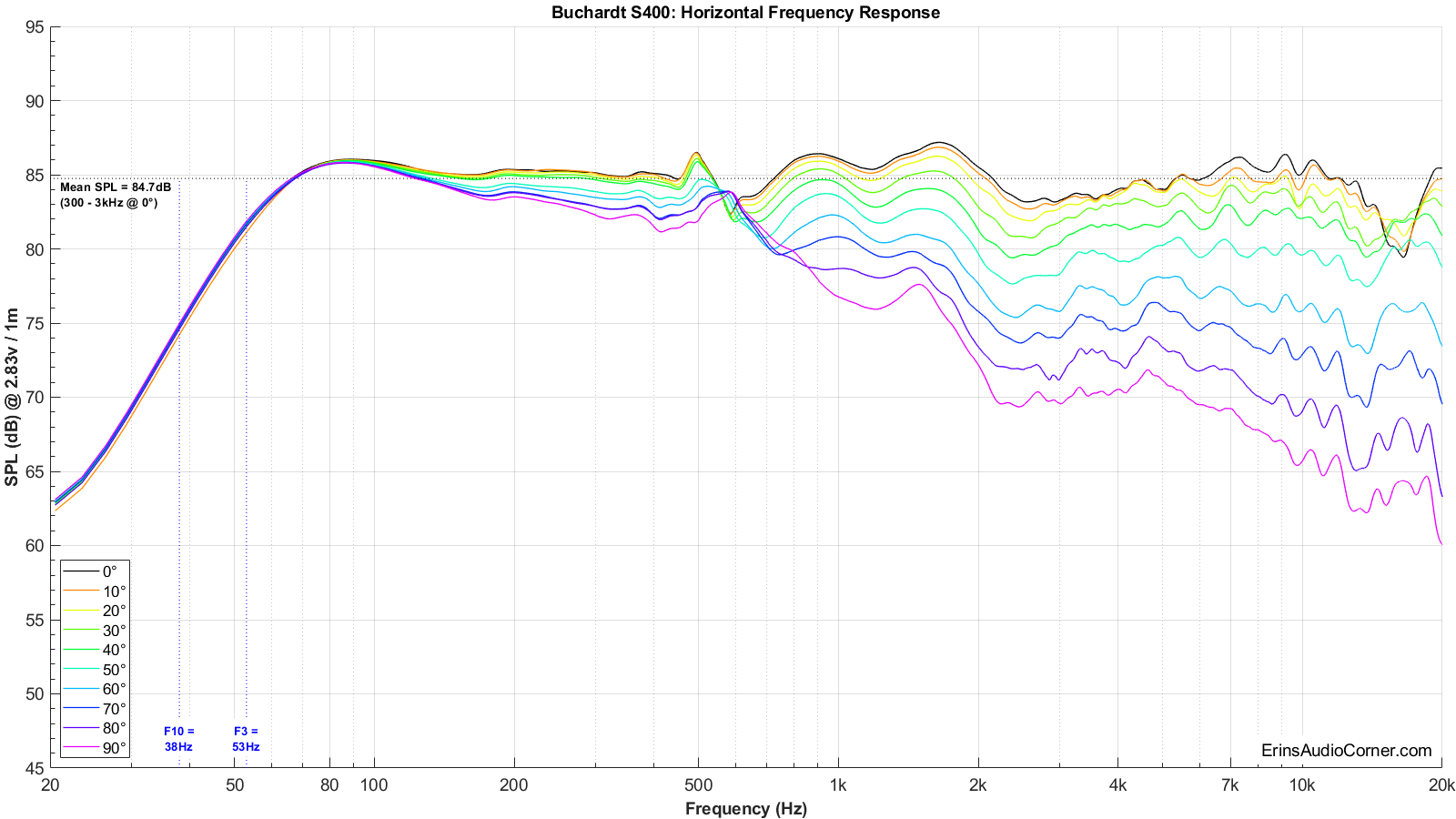
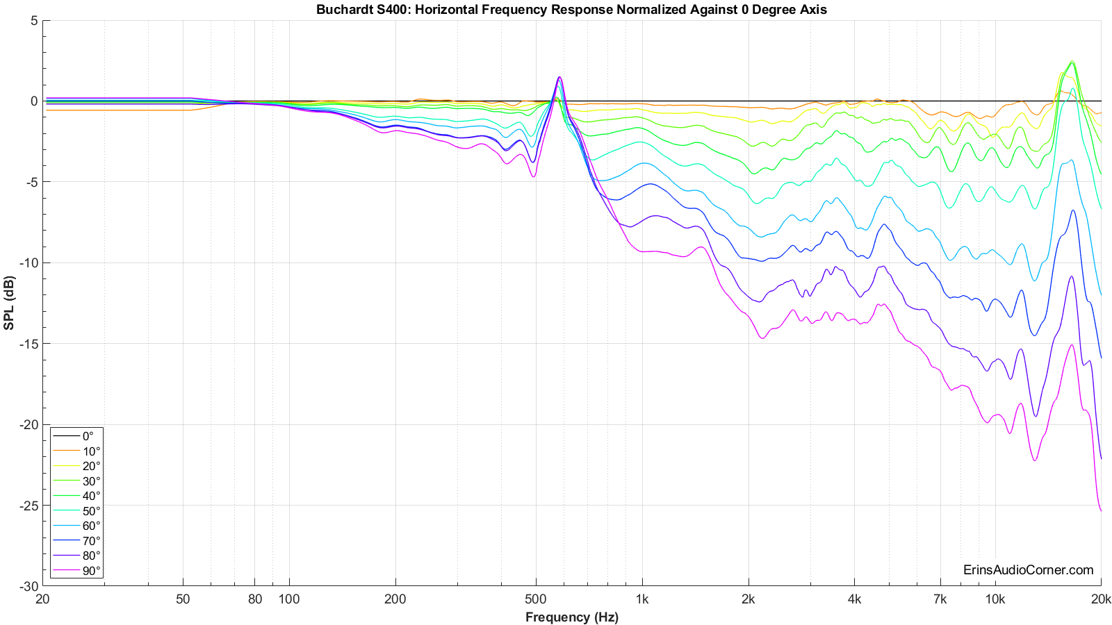
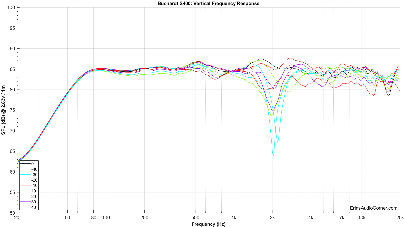
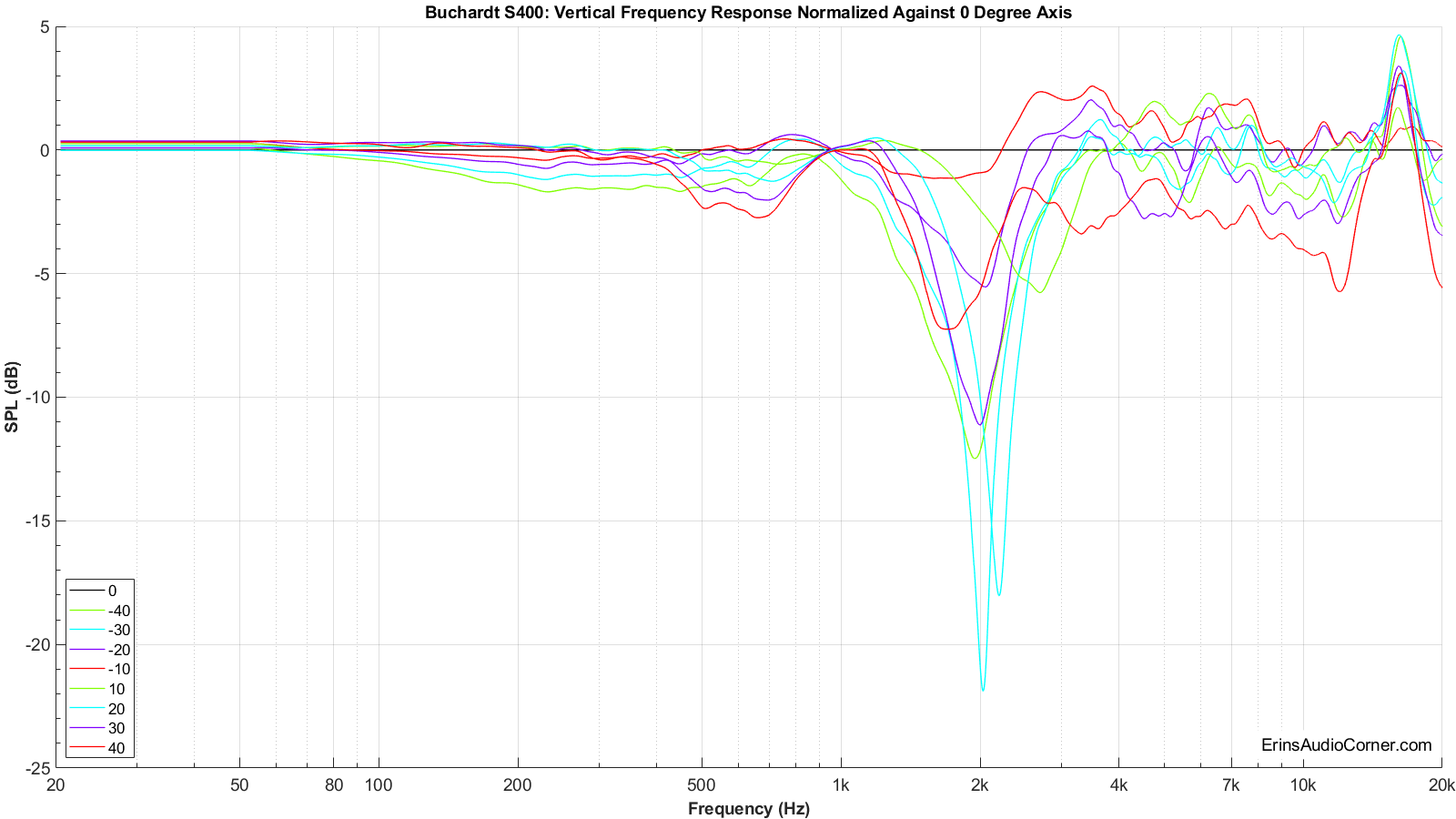
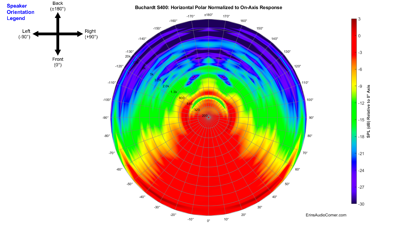
Below are both the horizontal and vertical response over a limited window (90° horizontal, ±40° vertical). I have provided a “normalized” set of data as well. The normalization simply means that I took the difference of the on-axis response and compared the other axes’ measurements to the on-axis response which gives the viewer a good idea of the speaker performance, relative to the on-axis response, as you move off-axis.

I know some will wonder about the apparent resonance around 500Hz. I didn’t find this objectionable in my subjective evaluations. Toole’s book covers threshold of audibility with various peaks, but I’ll reference this article for now: https://audioxpress.com/article/testing-loudspeakers-which-measurements-matter-part-1

Particularly, this section:

Figure 4 shows the detection threshold for resonances of various Qs in the presence of typical program music. You see that very narrow resonances (high Q) must be about 10dB above the average level to be heard, whereas very broad resonances need only be 1 to 2dB higher to be detected. This is fortunate because the limited resolution of quasi-anechoic responses may prevent you from seeing high Q peaks, but still allow you to find the lower Q resonances. The best way to identify resonances is via the cumulative spectral decay (CSD) discussed in the next section.

I pulled up my DSP software to determine what amplitude and Q shape would equal what I am seeing in the data. It took an Fo=500Hz, Gain = + 2.5dB and Q = 15 to match the measured Q. Meaning, the bandwidth of this peak is ~ 15. This is narrow Q with relatively low magnitude. So, while it looks offensive, it wasn’t to me and I believe the above quote backs up my notion that it wouldn’t be to others. Obviously, your mileage may vary. As far as the cause, well, there are no wiggles in the impedance measurement which would otherwise imply resonance. So, no resonance issue. Some may assume it is the enclosure (which is not braced) but the data doesn’t jive with that because, as you will see in the 360-degree horizontal radiation graphics below, this on-axis peak loses output as you move to the backside of the speaker. If it were caused by the side of the enclosure, I would expect the Q to have the same shape and amplitude as you move from the front to the back of the speaker. My educated guess is this is an influence of the passive radiator experiencing breakup, where on the backside of the speaker the passive radiator has already begun rolling off but on the frontside the pressure level of the mid/woofer combined with the breakup results in a narrow Q boost.

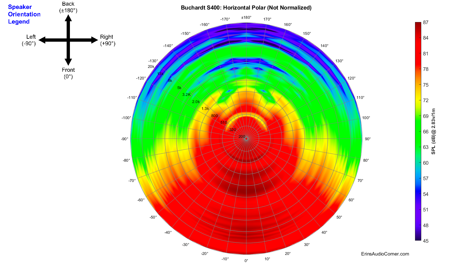
As I said above, the provided frequency response graphs were given with a limited set of data. I measured the response of the speaker’s vertical and horizontal axis in 10-degree steps over 360-degrees. Nearly 70 measurements in total are represented in my data. As you can imagine, providing all those data points in a single FR-type graphic below is a bit overwhelming and confusing for the viewer. A spectrogram is an alternate way to view this full set of data. This takes a 360-degree set of data and “collapses” it down to a rectangular representation of the various angles’ SPL. I have provided two sets of data: one set for horizontal and one for vertical. Each set consists of 3 graphics:

1. Full response (20Hz - 20kHz with the angles from 0° to ±180°) with absolute SPL values
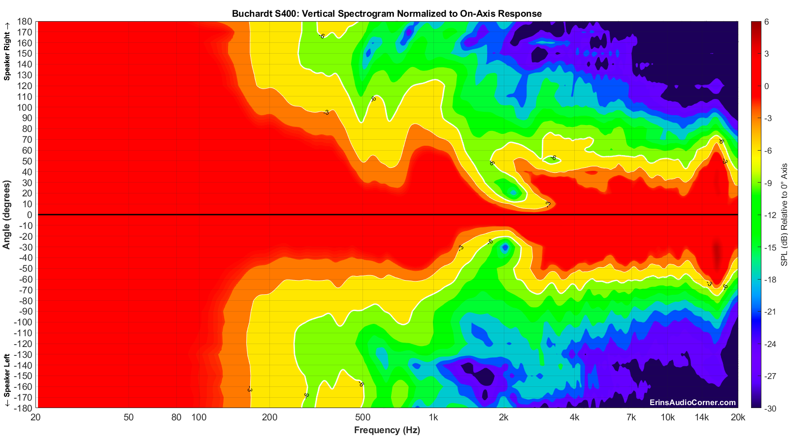
2. Full, “normalized” response (20Hz - 20kHz with the angles from 0° to ±180°) with SPL values relative to the 0-degree axis
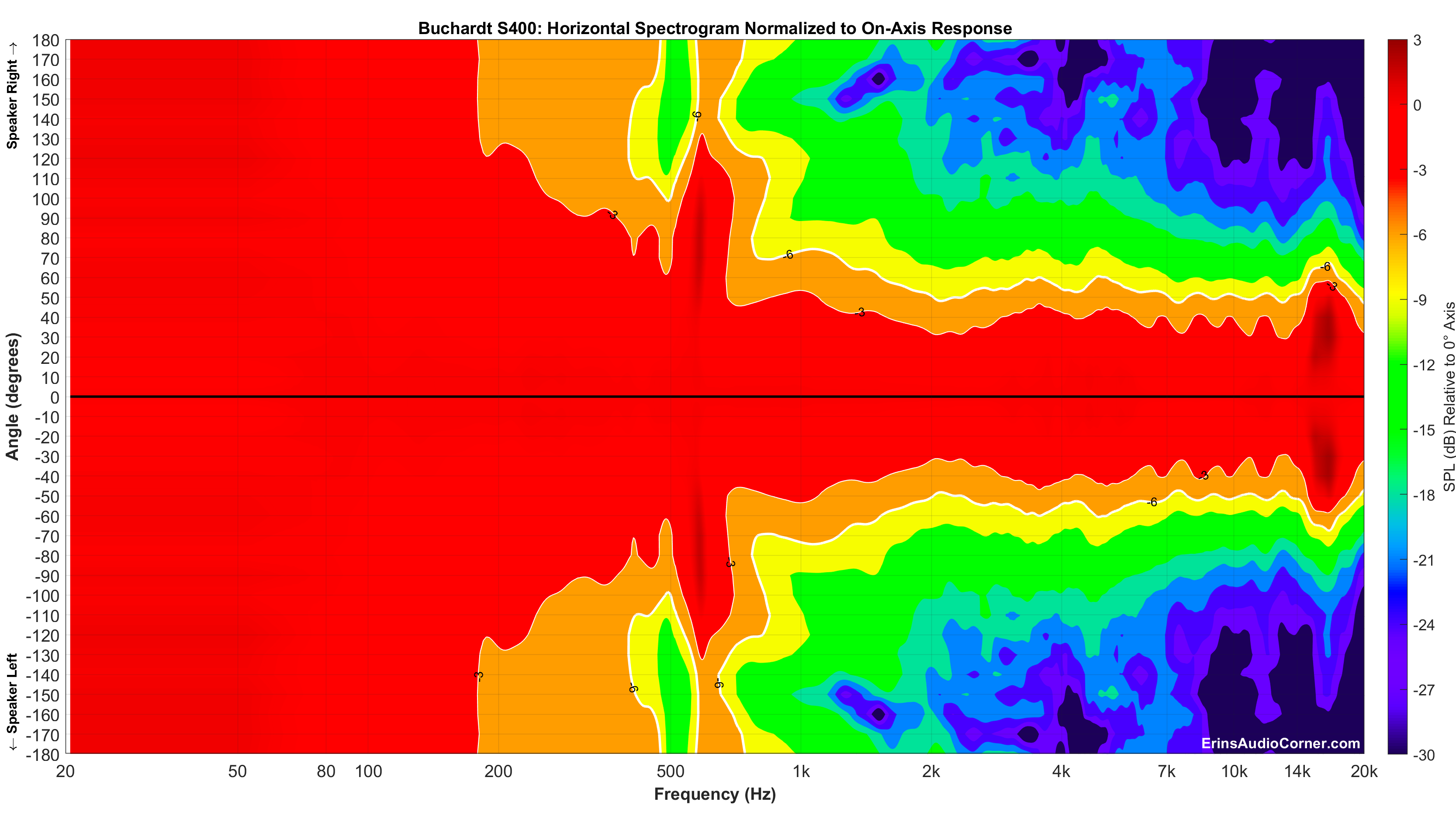
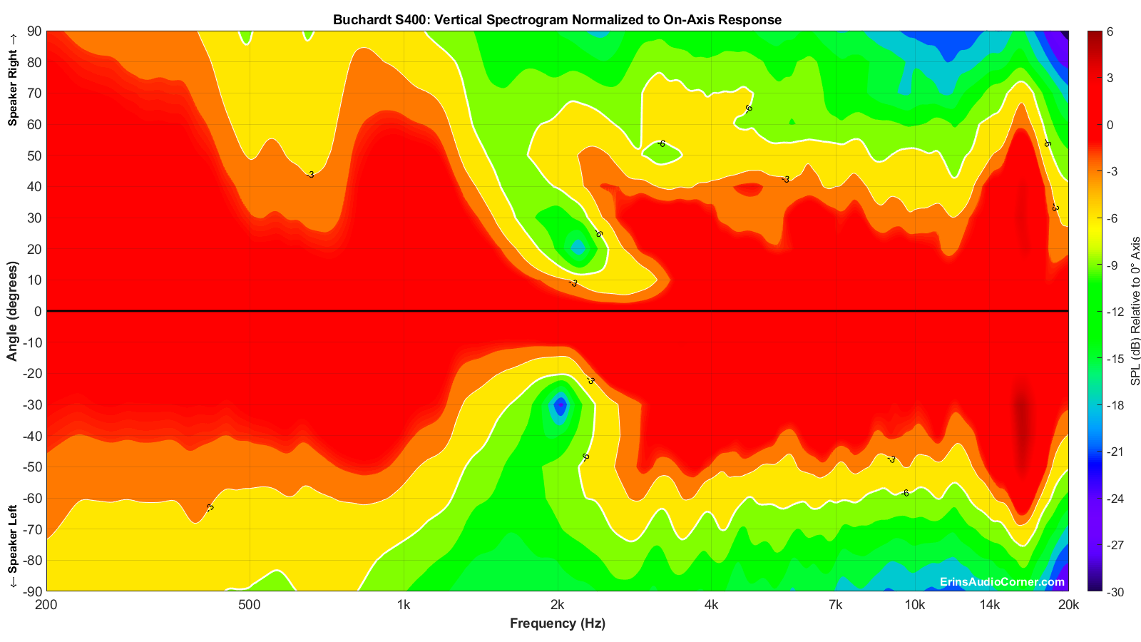
3. Normalized, “zoomed” response (200Hz - 20kHz with the angles from 0° to ±90°) with SPL values relative to the 0-degree axis

Normalized plots make it easier to compare how the speaker’s off-axis response behaves relative to the on-axis response curve.

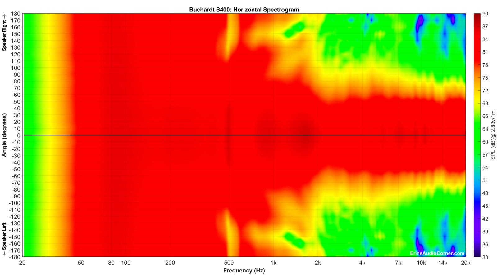
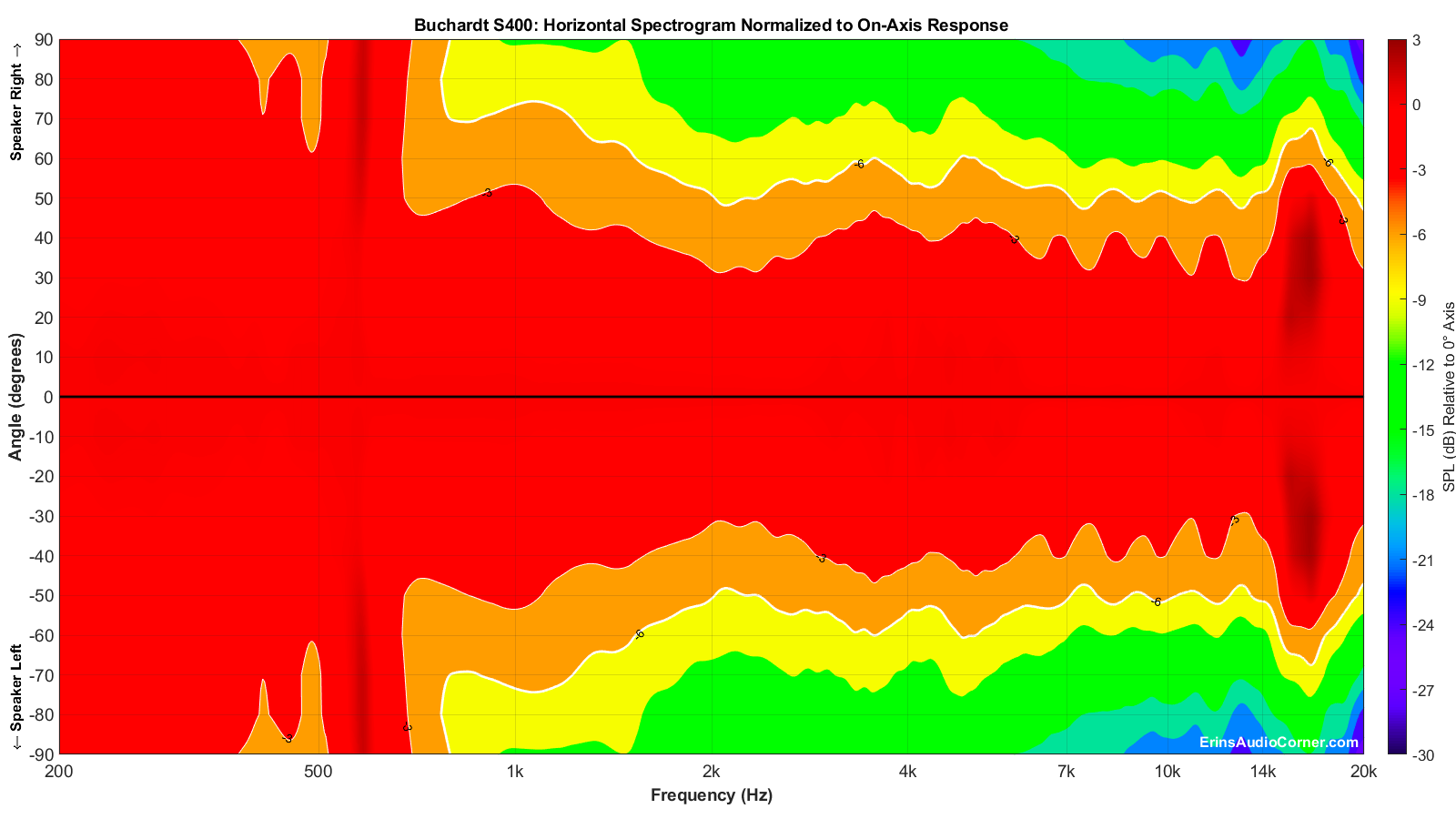
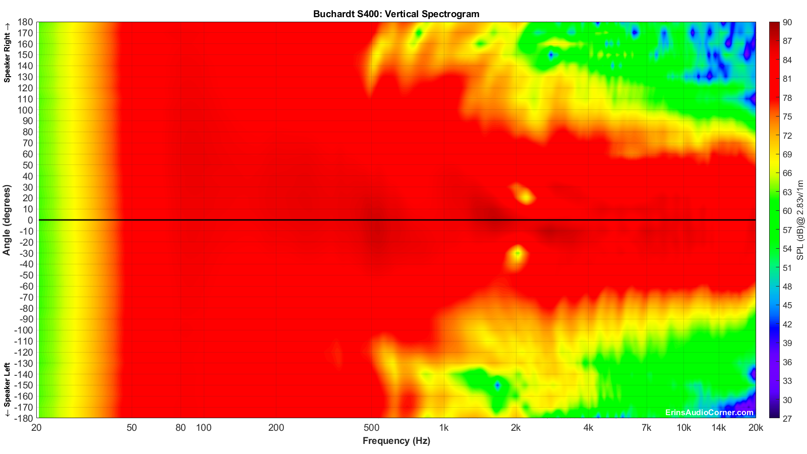
The above spectrograms are the standard way of providing directivity graphics by most reviewers. Some prefer not to normalize the data. Some prefer to normalize the data. Either way, it’s a useful visual to get an idea of the directivity characteristics of a speaker or driver.

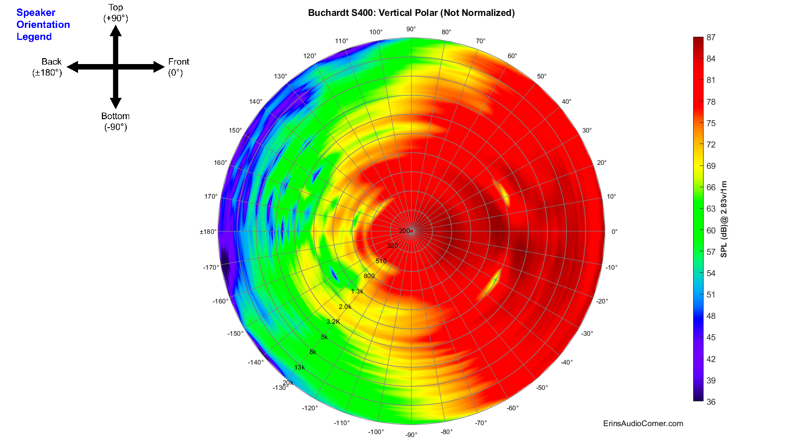
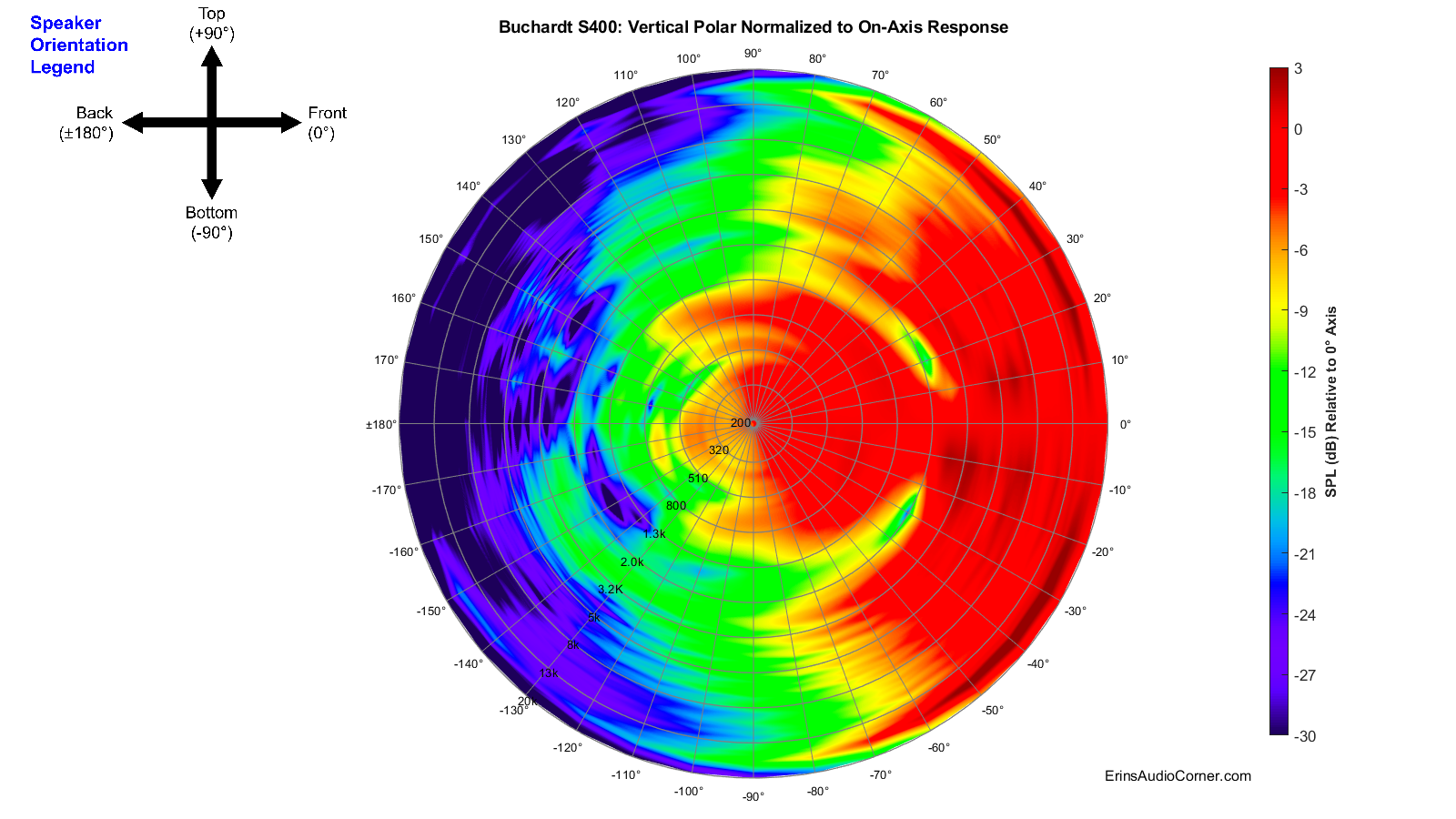
However, these “collapsed” representations of the sound field are not very intuitively viewed. At least not to me. So, I came up with a different way to view the speaker’s horizontal and vertical sound field by providing it across a 360° range in a globe plot below. I have provided both an absolute SPL version as well as a normalized version of both the horizontal and vertical sound fields.

Note the legend provided in the top left of each image which helps you understand speaker oreientation provided in my global plots below.

CEA-2034 (aka: Spinorama):

The following set of data is populated via the 360-degree, 10° stepped, “spins” from vertical and horizontal planes. Thus, this is sometimes referred to as “Spinorama” data. Audioholics has a great writeup on what these data mean (link here) and there is no sense in me trying to re-invent the wheel so I will reference you to them for further discussion. However, I will explain these curves lightly and provide my own spin on what they mean (pun totally intended). Sausalito Audio also has a good writeup on these curves here. Furthermore, you can find discussion in Dr. Floyd Toole’s book “Sound Reproduction”. Here’s my Amazon affiliate link if you want to purchase it and help me earn about 2% of the price. And, finally, here is a great video of Dr. Toole discussing the use of measurements to quantify in-room performance.

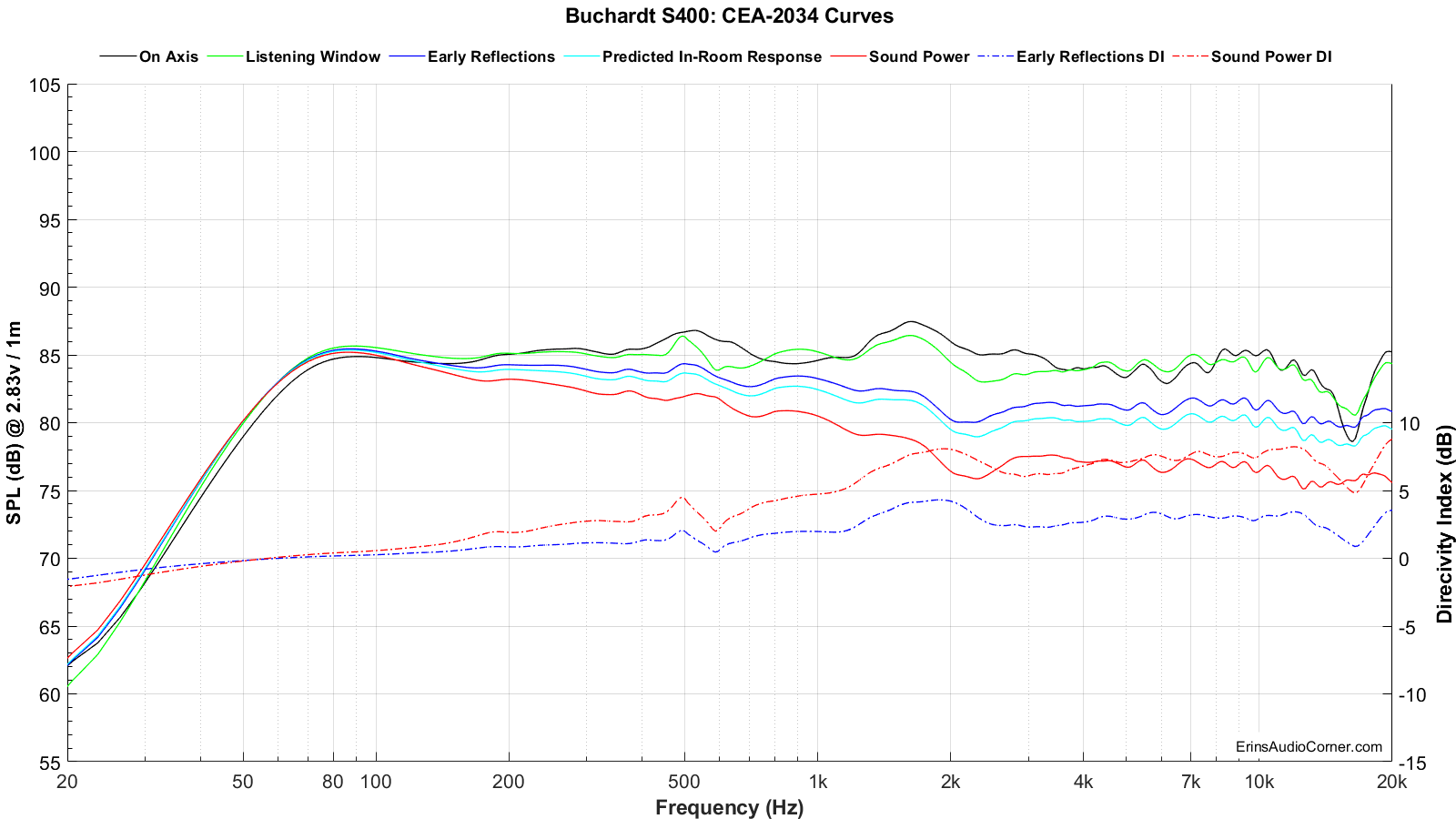
In short, the CEA-2034 graphic below takes all the response measurements (horizontal and vertical) and applies weighting and averaging to sub-sets and can help provide an (accurate) prediction of the response in a typical room. If there is a single set of data to use in your purchase decision, this is probably it.

Alternatively, click this arrow, if you want my quick take on what these curves mean without going to another site.

• On-Axis is simply the on-axis response. This is the 0-degree response curve.
• Listening Window is an average of the 0° to ±30° horizontal and 0° to ±10° vertical response curves and is used to understand what listeners typically hear in a home at the sweet spot, or Main Listening Position (MLP). The reason for this extended window of sound is simply because your room makeup might differ from another’s. This curve is an attempt to quantify a speaker’s performance over a smaller window that is often the norm for listening angle differences in various homes. It is important for this curve to very closely mimic the on-axis response. Deviations of the Listening Window curve relative to the on-axis response curve indicates a compromise in the speaker; often caused by directivity changes (as a speaker transitions from one drive-unit to another a la midwoofer to tweeter, or as a tweeter’s response becomes highly directional).
• Early Reflections is very useful because it helps us determine how the room’s influence will alter (corrupt, most of the time) the direct (on-axis) response. Ideally, the speaker radiates sound uniformly with no aberrations; no resonance, no directivity changes as the speaker transitions from the mid to the tweeter and so on. Because speakers often have these issues, however, what is reflected to us from the walls, ceiling and floor is not the same as what we hear from the on-axis, direct sound. And that’s a problem. Why is that a problem? As stated in Dr. Toole’s book “these are very influential in establishing timbral and spatial qualities”. Large deviations in this relative to the on-axis response also indicate areas where the room is of consequence. Also, it is important to understand the Early Reflections response is made up of rear-firing sounds. A speaker drive-unit is omnidirectional (radiating in all angles evenly) until the half-wavelength equals that of the drive-unit diameter. When the diameter is larger than the wavelength being played, the sound transitions from omnidirectional to directional; also known as “beaming”. Even tweeters beam. For example, a 1-inch dome tweeter will beam at approximately 6750Hz (speed of sound ÷ 2 ÷ diameter). In most speakers you have a single tweeter, firing forward. You can imagine that the high-frequency response in the front of the speaker would therefore be quite different than what is measured behind the speaker. So, being that the Early Reflections curve includes rear-hemisphere measurements you can understand that the high-frequency response would slope downward vs the on-axis response. This is understood and accepted.
• Predicted In-Room Response curve has the benefit of showing directivity mismatches at the crossover as well as resonances easily by comparing them to the overlaid Target curve (further down).
• Directivity Index (DI) curves are the difference in the Listening Window and the respective Early Reflections or Sound Power curves. My understanding, currently, is the Sound Power and Sound Power DI aren’t quite as useful for typical homes. However, there is emphasis placed on the Early Reflections DI curve. The right Y-Axis provides a value associated with the DI curves. The higher the number, the more directional the speaker. For example: a “0” DI curve - a curve which is completely flat - would be a speaker that is purely omnidirectional; radiating uniformly in all angles vertically and horizontally. A speaker that increases over frequency means that it is radiating in a tighter window as you increase in frequency. This is typical because, as I discussed above, even tweeters beam… and most speakers have a single tweeter facing the front and therefore, the speaker becomes directional at whatever the tweeter’s beaming frequency is. There isn’t necessarily a one-size-fits-all DI curve value. Though, it seems people (myself included) prefer a speaker with a wider soundstage which is found in lower directivity speakers (because more sound is bouncing off the side walls; which confuses the use of side-wall absorption but that’s for a later debate). However, what is important is that the curve, however tall you may prefer it to be, is smooth; almost linear. Dips and peaks mean that something, not good, is going on. But a linear curve indicates excellent transition through crossover regions, no resonance, etc. Since speakers are not perfect, though, linear DI curves are not the norm. Speakers become directional as they increase in frequency, around strong resonances, and as the sound transitions at the crossover from one drive-unit to another and you wind up with areas with peaks and/or dips whether they’re spread through a wide frequency range (low-Q) or very sharp/drastic (high-Q). But when you’re looking at the Early Reflections DI curve, look for this: smooth.

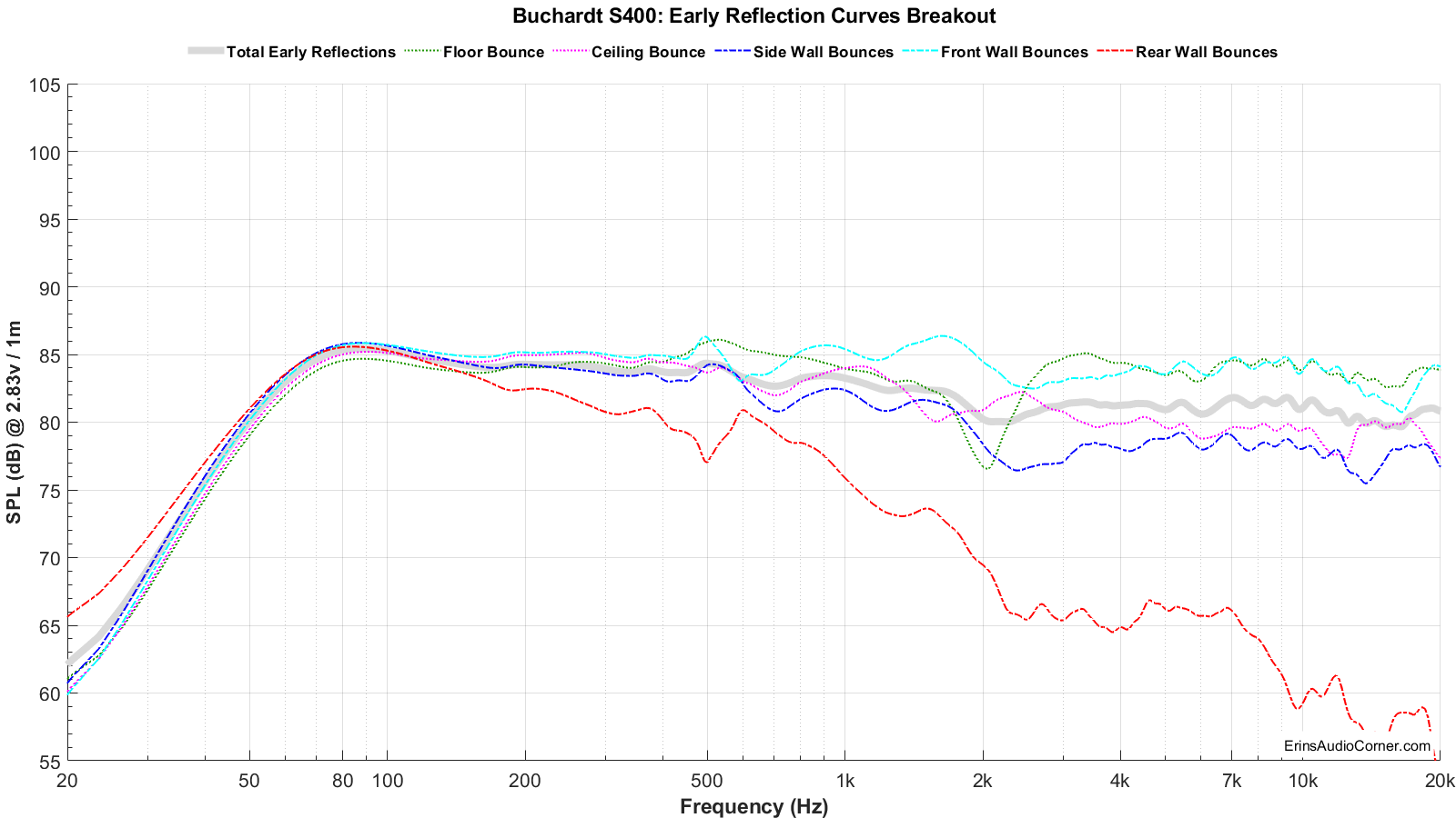
Below is a breakout of the typical room’s Early Reflections contributors (floor bounce, ceiling, rear wall, front wall and side wall reflections). From this you can determine how much absorption you need and where to place it to help remedy strong dips from the reflection(s).

And below is the Predicted In-Room response compared to a general Target curve equaling -1dB/octave.

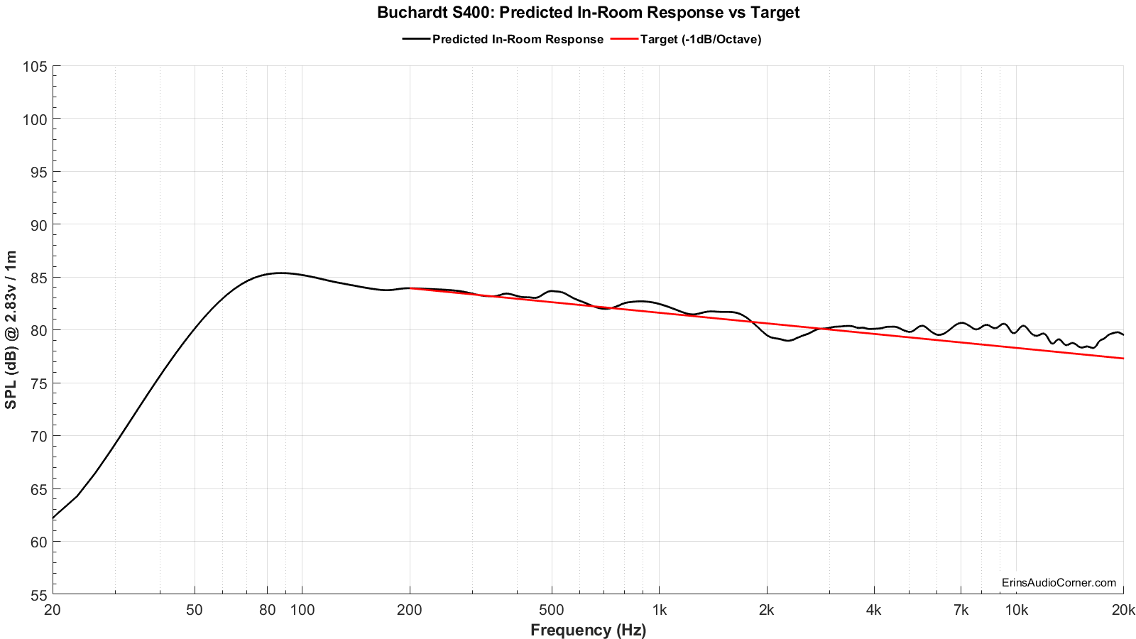
You may ask just how useful the above prediction is. Well, I’d be remiss for not delving in to that a little bit here. Please see my Analysis section below for discussion on this. :)

Total Harmonic Distortion (THD) and Compression:

Distortion and Compression measurements were completed in the nearfield (approximately 0.3 meters). However, SPL provided is relative to 1 meter distance.

Harmonic Distortion and Compression: What does this data mean? (click me for info)

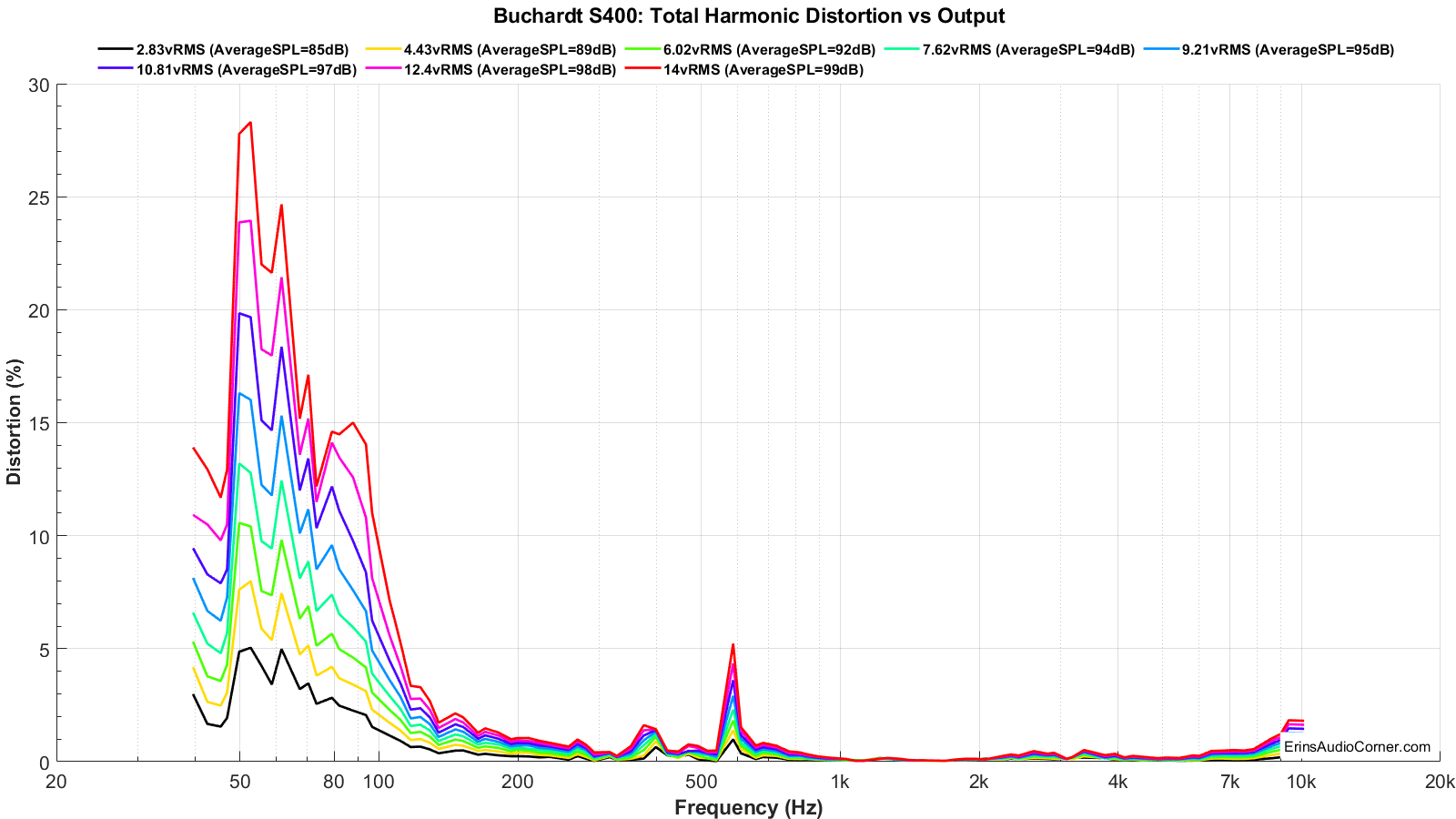
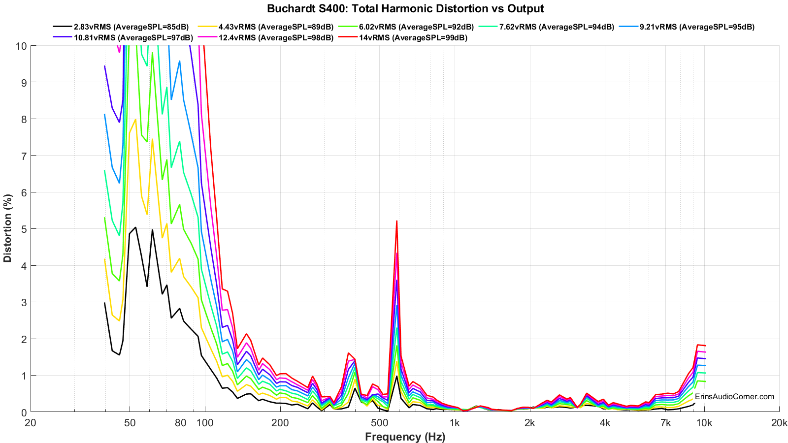
Harmonic Distortion and Compression are provided at varying levels to get an idea of what happens as the voltage into the speaker is increased and overall output volume increases. The “mean spl” values associated with each voltage provided in the legend is based on a calculation of expected volume assuming linear volume at the 300-3kHz region. Meaning, if a speaker is ideal and you tell your stereo to increase by 6dB by turning the volume knob +6dB, the output will increase by 6dB. In the real-world, however, a speaker is a mechanical device and there are compression effects that can limit the output volume and, therefore, you could possibly only get an actual increase in volume of 5dB. A good speaker will have little compression (< 1dB), where poorer speakers may suffer greater compression (> 2dB). Generally speaking, higher sensitivity speakers (like pro-audio speakers with 100dBSPL @ 2.83v/1m spec) suffer relatively no compression while lower sensitivity speakers (low 80’s dBSPL @ 2.83v/1m) suffer more compression. When a crossover is used the compression near the speaker’s Fs is attenuated and overall the compression effects are mitigated. With that in mind, what you see below is first the Total Harmonic Distortion at varying output levels.

What you see below is first the Total Harmonic Distortion at varying output levels. At 2.83vRMS the mean SPL is about 86dB at 1 meter (over 300-3kHz). Distortion at this output is mostly under 0.50% above 200Hz and hits the 3% mark at about 80Hz. As you’d expect, the distortion increases as volume increases. Namely, near the speaker’s roll off point.

However, based on a poll I conducted, most people’s in-room listening distance is between 3 to 4 meters from their speakers at a volume of about 85dB to 90dB. Few people realize just how loud 90dB is. I’ve often found people tend to overestimate their listening levels by a fair bit. But, for the sake of determining how these speakers perform at the higher end of music listening, let’s assume the following: 1) you are in your room and about 4 meters (~ 13 feet) from the speakers and 2) you listen to these speakers at about 90dB at the listening position. In this scenario, you will need to look at the 93dB (6.02vRMS) measurements for THD and Compression. Why? The measurements I provide are, again, referenced to 1 meter distance from the speaker and of a single speaker. To get to 4 meters you double the distance twice (1 meter to 2 meters, 2 meters to 4 meters. Each time you double the distance you increase or decrease the SPL level by ±6dB (+6dB if you move toward the speaker; -6dB if you move away). This math gets you to 90dB target + 12dB for one speaker at 4 meters. But you’d listen to a pair of speakers in a room which results in +3dB (for doubling of speakers). Now you’re at 90+12+3dB. Also, typical rooms have a +6dB gain. So, in order to get from 90dB at 4 meters in-room for a pair of speakers to the SPL at 1-meter for a single speaker in anechoic conditions to match my measurements: the math breaks down as: 90+12-3-6dB = 93dB for the single speaker at 1 meter. Using the 93dB measurement tells you the measured low-frequency distortion at about 80Hz is near 6% THD. Will you hear that? Pure distortion is more subjective and depends not just on the listener but also no the program material. However, in this case, the distortion increase is due to the mechanical limits of the speaker. And it was audible. I verified this myself and will discuss it in my analysis section. But, remember, this speaker test is done without a crossover of any sort. Once you add a crossover the distortion would naturally decrease.

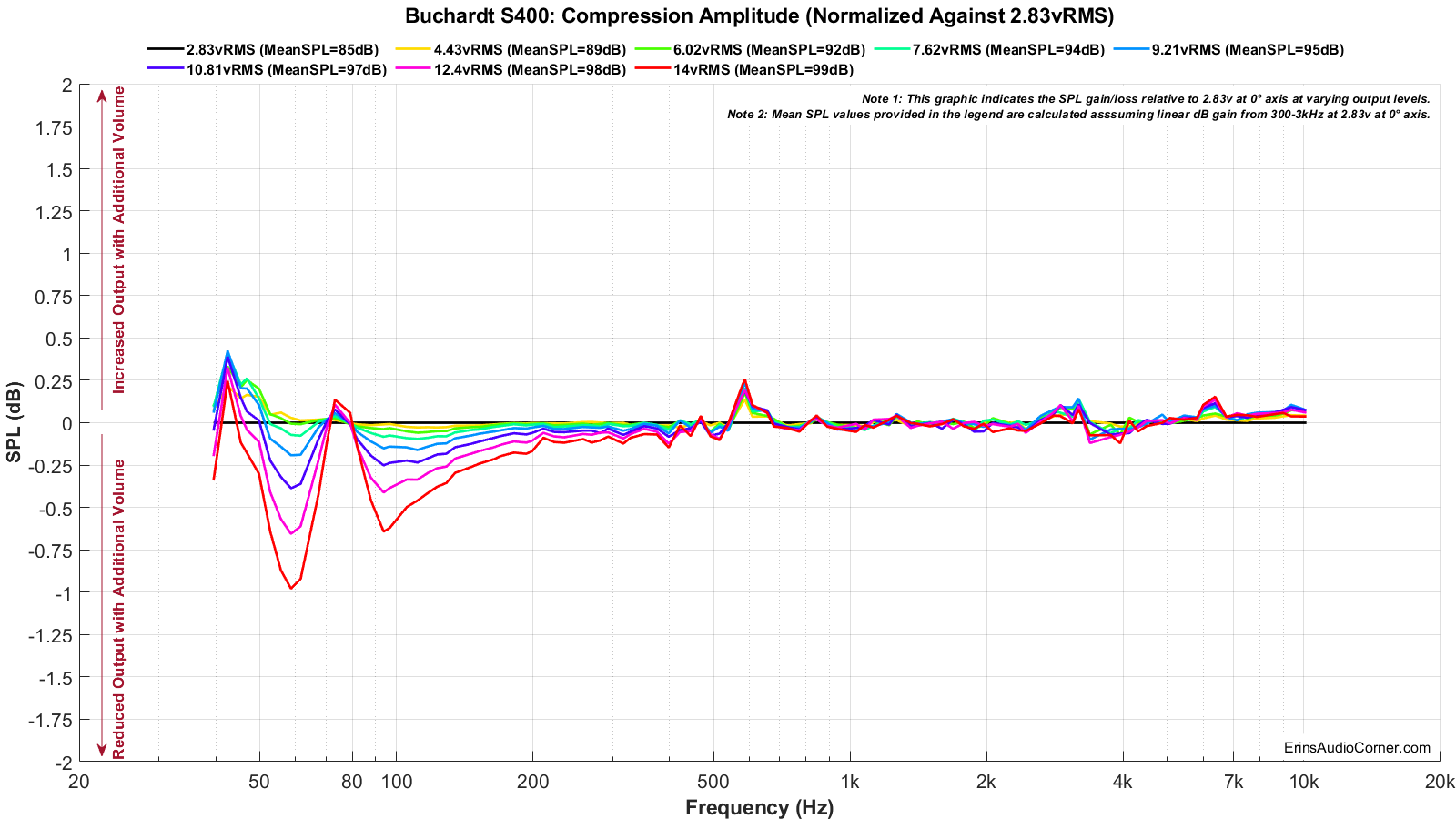
The compression effects shown in the image below are a visual way of seeing just what happens as the volume is increased. This one is straight-forward. Take the legend’s SPL value and add or subtract the data from the graphic. This tells you if you’re losing or gaining output (yes, you can gain output from compression; as un-intuitive as that seems). Mostly, the compression results in a loss due to temperature increase in the voice coil of the drive unit. Let’s look at a specific example. Take the 90dB at 4 meters target listening volume provided above. Again, you need 93dB’s (6.02vRMS) data. At that volume, the highest amount of compression measured is about 1/10dB. Nothing, really. At worst, this speaker experienced about 1dB of output loss at about 60Hz with 14vRMS. The average SPL of this speaker at 2.83vRMS was 86.5dB between 300Hz-3kHz. 14vRMS relates to 100dB mean SPL. So, a gain of about 13.5dB. This means at 60Hz you lose 1dB and therefore wind up with only a 12dB gain over the 2.83vRMS measurement provided at the top of this review. And at a listening distance of 3 meters that would be about 103dB (or 102dB with this 1dB loss in compression at 60Hz). This is a small bookshelf speaker. I’d say this output level is certainly reasonable.

Extra Measurements:

These are just some extra sets of measurements I completed. Some, I didn’t process through my MATLAB scripts so they’re kind of raw. But I know some would like to see them so here you go.

Grille on vs Grille off.

Moral of this story? Leave the grille off. At 90° off-axis it looks worse (not pictured).

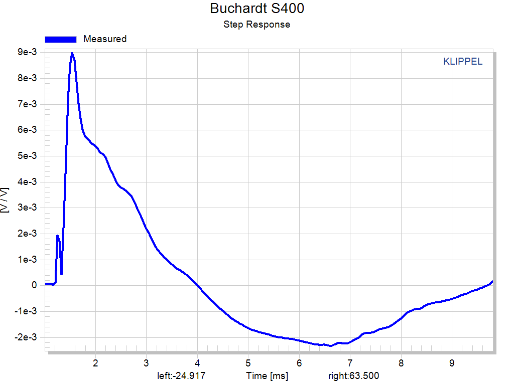
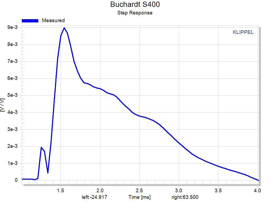
Step-Response.

One not zoomed and one zoomed.

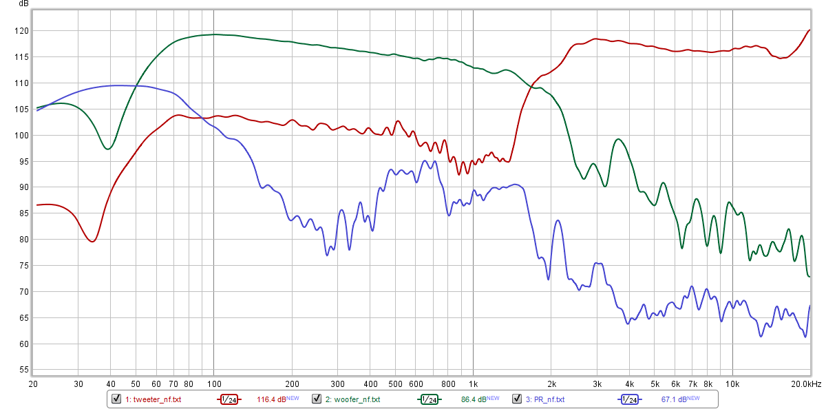
Nearfield measurements.

Note: These are not relative at all. I just placed the mic near to the respective driver/enclosure and swept the signal. The tweeter SPL is not absolute, nor is mid/woofer or passive radiator. So, these are not to be used directly against each other. Don’t use this to try to determine crossover frequency. Just more of a “humph” bit of information. Got it? Good. I do want to mention the increased output in the passive radiator (blue) between 400-700Hz. I believe we are seeing these effects in the 500-600Hz range; the 500Hz resonance I discussed earlier.

Objective Evaluation:

Now that we have this over-abundance of frequency response data, let’s do something different. Let’s compare the data to what the manufacturer says about their own product and see if my objective data backs this up. Don’t worry, we will get to the subjective analysis shortly.

Buchardt’s site states:

“S400 keeps and controls the directivity from 1000 Hz and all the way up.” “What this translates to is a non-distorted, evenly distributed in-room frequency response that allows the S400’s to sound balanced even at extreme angles, which in turn allows the enthusiast to enjoy sundry benefits like improved imaging, a bigger soundstage, and better transparency. This excellent off-axis response will also result in a drastically widened ‘sweet spot’ and most importantly, a character that will remain steadfast even as you move around your home as the music plays.”

Well, let’s see…

The normalized horizontal 360-degree radiation pattern provided above shows that the response between ±40° is even throughout. This means that what you hear between -40° and +40° will be roughly the same. So far, this jives with what the mfg. states. What happens when you put the speakers in a room, though?

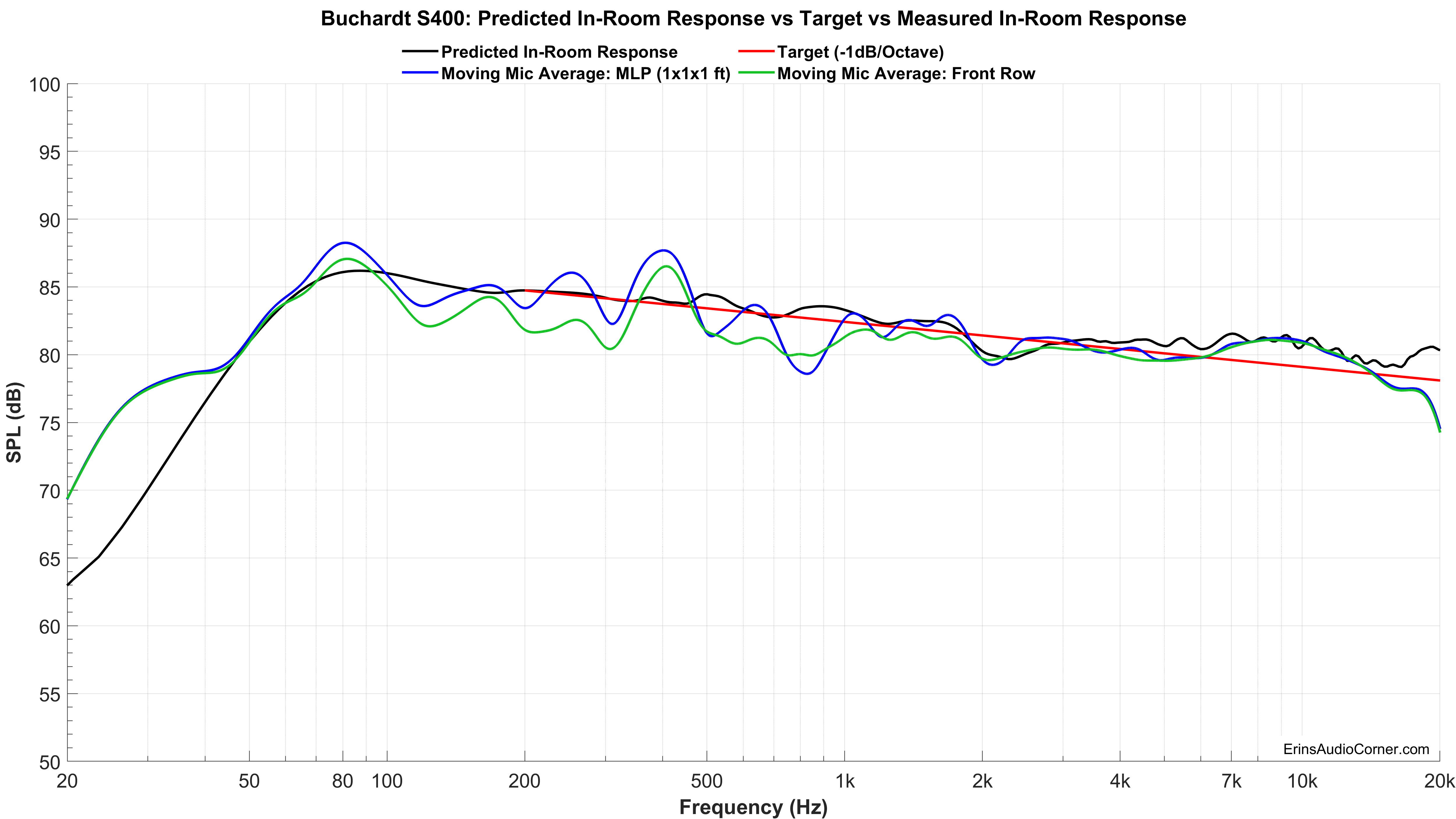
The above is a set of measured in-room response curves from my home theater vs the predicted in-room response curve (black). My home theater response measurements were captured via a Moving Mic Method while using Room EQ Wizard’s (REW) “averaging” function while playing Pseudo Pink-Noise. I measured a small window at the Main Listening Position (MLP) (blue) as well as the response over the entire front row (about 6.5 feet wide from end to end listening positions) (green). I overlaid these averages on a target curve equaling -1dB/octave from 200Hz to 20kHz (red).

What stands out to me is how alike the response of the MLP measurement (single seat) vs the ENTIRE front row measurement is above 1kHz. The two vary by only about 2.5dB from 1-2kHz, less than ~1dB from 2-4kHz and above 5kHz they are practically the same. That’s very impressive! I’d say Buchardt’s above quote is verified. Kudos to them!

Another quote from Buchardt’s site:

As an example, larger tweeters tend to be popular because of their power handling and frequency bandwidth, which allows them to be crossed over at lower frequencies. The caveat is that these larger tweeters do not tend to sound as good off-axis and, subjectively speaking, do not sound quite as good (to our ears) as a smaller, well-engineered tweeter. For us, it’s all about performance. And when you get right down to it, the 19mm tweeter that we use fits our goals perfectly.

For one, the measurements are about as ideal as we’ve found. Secondly, the off-axis performance is tremendous. Any of the limitations that would normally come from using this tweeter has been mitigated by our deep waveguide. The result is exactly what we were looking for. Top end that’s effortlessly free of distortion, resulting in a presentation that’s clean, detailed, powerful, and perfectly integrated with the rest of the speaker.

Well, looking at the Total Harmonic Distortion graphs and the already-mentioned front-row measurements I’d say I agree with all of this. Certainly, when one uses a smaller tweeter the concern with distortion increases (ha! no pun intended!). But, as you can see from the THD data I’ve provided, this is of no concern. Even at output levels where the speaker’s woofer exceeds mechanical limits, the tweeter is still strumming away. Heck, at 100dB @ 1 meter the distortion between 2-3kHz (the crossover region) is below 0.50% THD. They did a good job here.

I think Buchardt’s marketing page here is pretty honest. So, now let’s do some of our own analysis. Doubling back to the 360-degree globe plots we can see how the speaker’s response behaves on and off-axis (as well as off-axis relative to on-axis via the normalized plots). We can also use all the other FR-based and Spinorama plots (specifically the Early Reflections) to help solidify our understanding. Start with the horizontal. Looking at the non-normalized plot we see a few things:

1. High-Q resonance at about 500Hz (discussed earlier)
2. Low-Q resonance at about 800: low directivity impact so may not be as bothersome
3. Low-Q resonance at about 1.6kHz: 2-3dB increase in directivity here followed by dip near crossover region; smooths out in Early Reflections curve but also shows up as a potential issue via the Predicted In-Room response vs Target. I believe I heard this, being next to the 2-3kHz dip I noted in my Subjective Evaluation below.
4. Shelf-like peaking from ~ 7-10kHz spreading the angles from ±30°. This was audible to me (see Subjective Evaluation section).

Moving on to the Vertical Response we see a clear directivity mismatch between 1-3kHz, presumably where the crossover is placed. What this means is you have a decreased “window” where the response, vertically, will behave in the same manner as you move up/down. Typically, when we look at FR data we tend to ignore the vertical response other than in the tight ±10° window, accounted for in the Listening Window curve provided earlier. But we shouldn’t. It plays a role in the Early Reflections curve, as discussed previously and you still want a good match here. However, the speaker still behaves uniformly in the ±10° vertical window which bodes well for the Listening Window curve.

Subjective Evaluation:

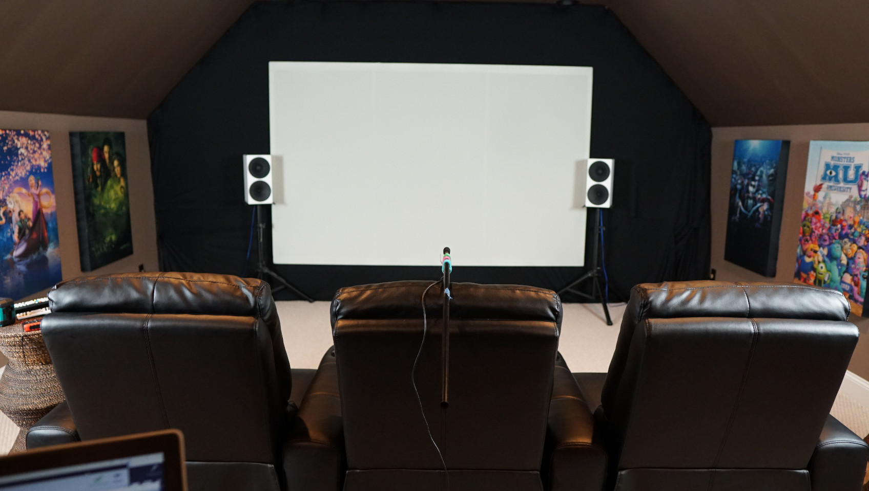
Before I dive in to using hyperlatives (hyperbole + superlatives) let me first give you the layout of my room…

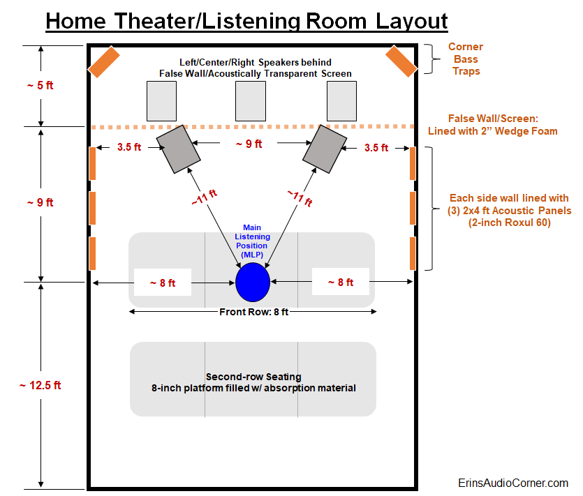
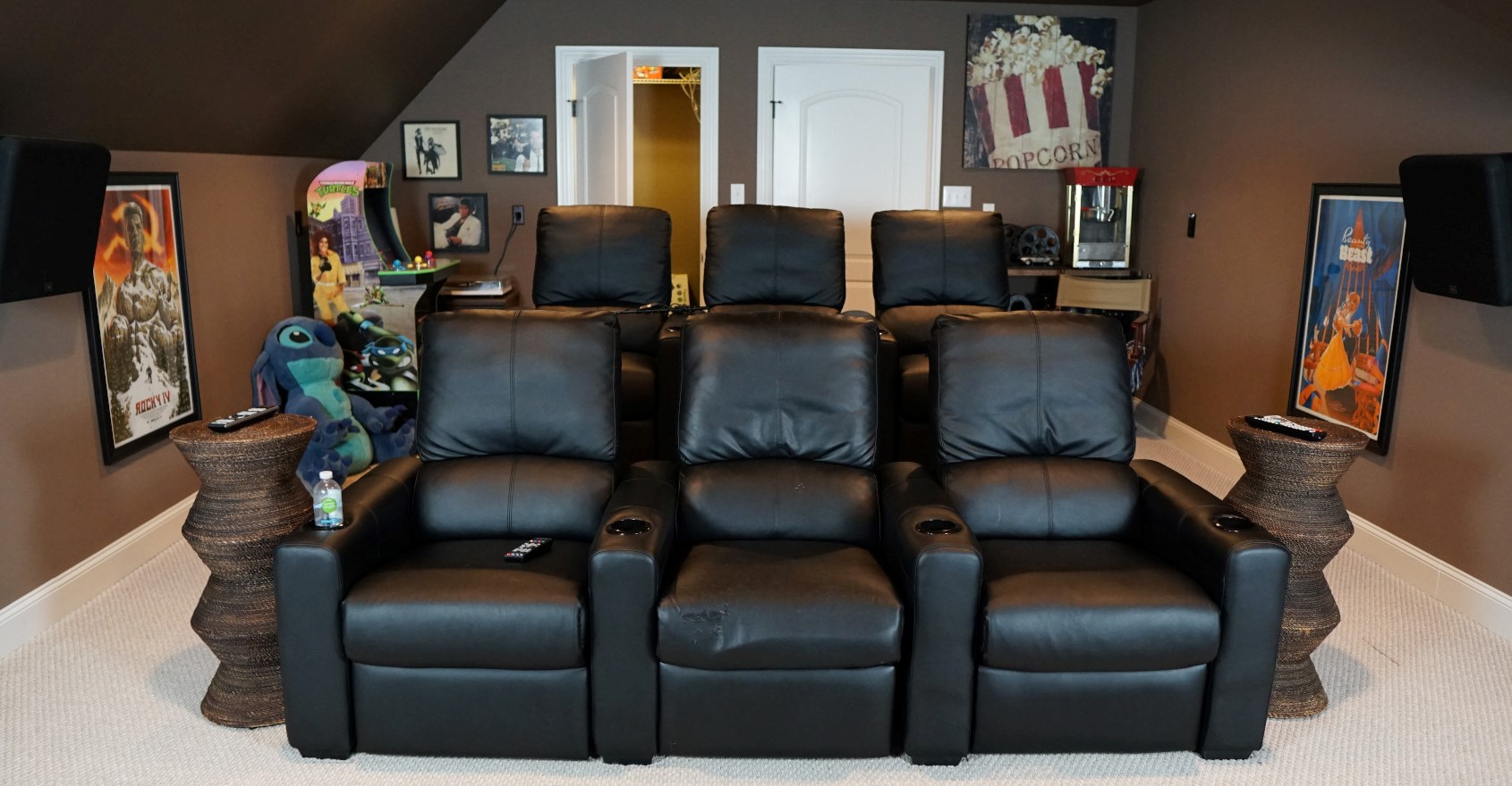
Note the distance from speakers to Main Listening Position (MLP) is approximately 11 feet.

If the false wall part is odd to you, here’s some background. I don’t like seeing speakers when watching a movie. So, I built a false wall and used an acoustically transparent screen with speakers behind it. The wall is only 2x4’s; no panels of wood or anything. Just a skeleton of a wall to give me something to attach the screen and acoustic treatment to. There is 2-inch wedge foam affixed to the 2x4 studs and between the false wall and back of the room are the front speakers (L/C/R & 18-inch subwoofers).

My demo music:

Title	Artist	Album
Let It Whip	Dazz Band	20th Century Masters: The Best Of Dazz Band
These Dreams	Heart	Heart (MFSL)
Cherry Bomb	John Cougar Mellencamp	The Lonesome Jubilee
I Don’t Care Anymore	Phil Collins	Hello, I Must Be Going!
Enjoy The Silence	Depeche Mode	Best Of Depeche Mode, Vol. 1
Higher Love	Steve Winwood	Back In The High Life (MFSL UDCD-611)
24K Magic	Bruno Mars	24K Magic
Magic	The Cars	Heartbeat City (MFSL)
Something About You	Level 42	The Very Best Of
Everlasting Love	Howard Jones	The Best of Howard Jones
Everybody Wants To Rule The World	Tears for Fears	Songs from the Big Chair (2014 Deluxe Edition - Disc 1)
Head Over Heels/Broken	Tears for Fears	Songs from the Big Chair (2014 Deluxe Edition - Disc 1)
Know Your Enemy	Rage Against The Machine	Rage Against The Machine (Hybrid SACD)
You’re My Best Friend	Queen	A Night at the Opera
Heartbreaker	Pat Benatar	In the Heat of the Night (DCC)
Doo Wop (That Thing)	Lauryn Hill	The Miseducation of Lauryn Hill
The Way You Make Me Feel	Michael Jackson	Bad
You Don’t Mess Around With Jim	Jim Croce	24 karat Gold In A Bottle (DCC)

Note: I don’t generally audition speakers with the typical “audiophile” music. I have thousands of high-quality albums ranging from pop to metal to jazz and all around. I don’t typically listen to “audiophile” music because I just don’t enjoy it. It is far more important that your evaluation music be something you are familiar with than it is to be esoteric for the sake of being esoteric. You also want to listen to music you enjoy because auditioning a stereo system shouldn’t feel like a chore. Such is the case in my evaluations. Besides, the subjective evaluation is purely to help tie to the objective data and make sense of what I am hearing to help you all get an understanding of how relevant the data is. As you will see below, my music selection did a great job at providing enough range for me to identify the issues that readily appear in the data.

Subjective Analysis Setup:

• The speaker was aimed on-axis with the tweeter at ear level.
• I used Room EQ Wizard (REW) and my calibrated MiniDSP UMIK-1 to get the volume on my AVR relative to what the actual measured SPL was in the MLP (~11 feet from the speakers). I varied it between 85-90dB, occasionally going up to the mid 90’s to see what the output capability was. In a poll I found most listen to music in this range. Realistically, 90dB is loud for long-term listening volume and I find most overestimate their listening volume until an SPL microphone is used to determine the actual level.
• All speakers are provided a relatively high level of Pseudo Pink-Noise for a day or two - with breaks in between - in order to calm any “break-in” concerns.
• I demoed these speakers without a crossover and without EQ.

I listened to these speakers and made my subjective notes before I started measuring objectively. I did not want my knowledge of the measurements to influence my subjective opinion. This is important because I want to try to correlate the objective data with what I hear in my listening space in order to determine the validity of the measurement process. I try to do a few listening sessions over a couple days so I can give my ears a break and come back “fresh”. I also want to be as transparent to you as I can be so below are my subjective evaluations made before I began any measurements.

You may notice that I am more descriptive of frequencies than sounds. Many reviewers will quantify their evaluation discussing how a tone sounded or an instrument sounded. My history has always been in relating the sounds to frequencies so I can understand where I need to EQ. So, I’m no good at telling you a cello didn’t sound like it should with a certain fellow of a certain weight playing it. I just go off relative sounds, basically evaluating performance by “How does this frequency sound compared to another”. But I use this method along with this Interactive Frequency Chart and it works out in the end.

Let’s look again at the measured in-room response I provided above:

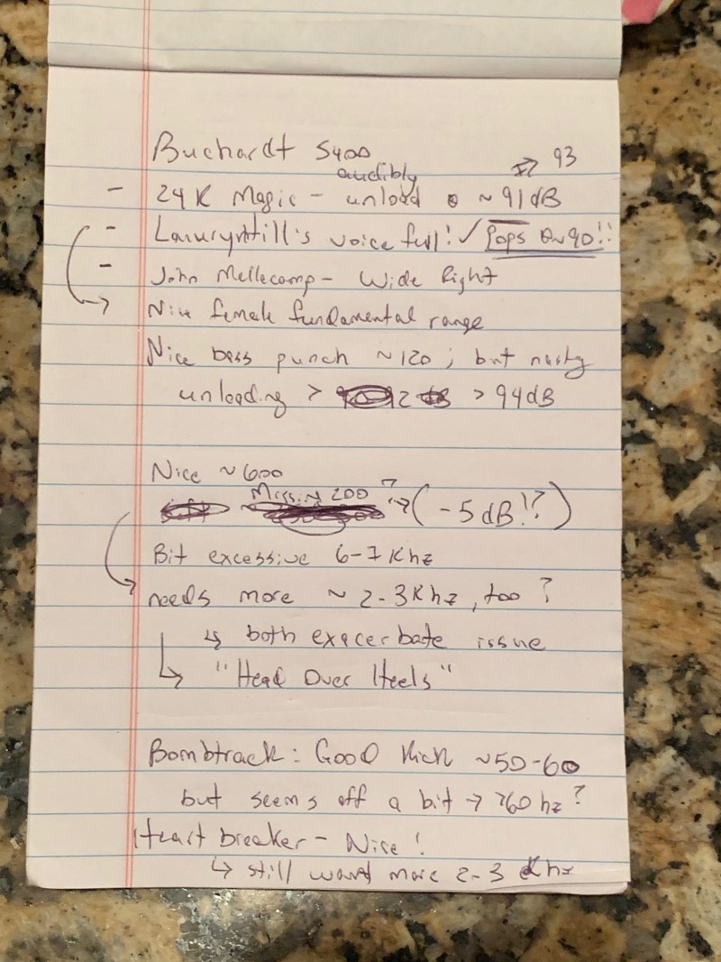
Here’s the rundown of my subjective notes (in quotes) and where it fits with objective:

• Naturally, the lack of a high-pass filter (HPF) limited the maximum SPL I could achieve and I noticed audibly unloading of the woofer/passive radiator at volumes in the low 90dB range; more so with the Lauryn Hill and Bruno Mars tracks because they are a bit more stressing on the low end. When I implemented a HPF = 80Hz/24dB the issue was diminished, and I could eek out a couple more dB in output. But, overall, my maximum in-seat SPL was about 95dB @ 11 feet even with the 80Hz/24dB crossover. Per the “6dB/doubling of distance” rule, if you are seated at about 5.5 feet that would increase to 101dB.
• I liked that the John Mellencamp track was wide right as expected but did so without also coming forward of the soundstage which is a positive (some speakers throw the image at an angle forward rather than forward and to the side).
• Female fundamental vocals were nice around 250Hz.
• Male fundamentals were a bit thin around 200Hz.
• The image was locked in even when moving my head around in the listening position.
• Too much 6-7kHz, per my notes. But I’d also say that covers the 8kHz range. In other words, the speaker was a bit “hot”. Not terribly so. Just a few songs accentuated the upper treble range more than I felt it should have been. The data backs this up as well: look at the 6-8kHz region in the Predicted In-Room Response vs Target vs Measured. It’s elevated throughout; extending into the extreme high frequencies.
• The 2-3kHz region was lacking in presence. Some vocalists (namely, males) sounded a bit “behind” the music. I don’t know if this is due to the lower level in the 200Hz region or a combination with this perceived 2-3kHz dip. Apparently, I noticed this most on “Head Over Heels” by Tears For Fears. This could be caused by the directivity mismatch between the mid/woofer and the waveguide (as evidenced in the spectrograms where the response loses output as it transitions from speaker to speaker at the crossover point).
• I wrote that there was good kickdrum in Bombtrack (Rage Against the Machine) but “seems a bit off > 60Hz”. This is likely the unloading I was hearing, mentioned in the first bullet above.
• Again, very wide sweet spot in the high frequencies. I’m very impressed by this. The room is still your enemy below about 400Hz in most rooms so there’s not much a speaker of this smaller size can do to help control directivity above 1kHz (you’d need a HUGE waveguide to control directivity down to 400Hz. I know, I have some as part of my theater setup and they only control down to 500Hz).

Now, once I ran Dirac Live using the MiniDSP DRC88A I got rid of some of the room modes shown above, having Dirac do no correction above 800Hz so I would still get the “speaker response” instead of it being dominated by the room as well. I also ran a full-correction from 20-20kHz and that smoothed out the 6-8kHz issues I mentioned. You can see the Dirac measured responses (blue), the Dirac target curve (orange) and the corrected Dirac response (green) below.

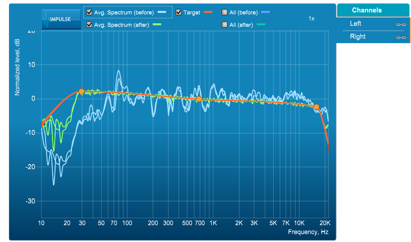
This helped smooth the 400Hz bump you see in my in-room measurements above. This also helped improve the male fundamental complaint I had. Though, it didn’t resolve it entirely. Looking back at the data I see the slight bump in bass around 100Hz with a mild dip in the 160Hz region. I can’t help but wonder if the 160Hz region isn’t the region that I didn’t feel was not as full as it should have been and causing my complaint about male vocals being “thin”. You can see that Dirac also brought down the bump between 6-8kHz (and beyond) which was a welcomed improvement to my ears. Dirac extended the bass while knocking down the peak at 80Hz. This made a significant improvement to the sound, but as I mentioned earlier, there is a maximum output to these bookshelf speakers and with the DSP effectively boosting the lower frequencies, I wound up having to use a crossover at higher volumes. But, for lower listening levels (< 85dB) it was impressive to hear how low these speakers played, and they sounded great doing it after Dirac smoothed things out.

As an aside, you don’t have to have Dirac Live to enjoy a speaker. But with all the problems the room itself creates, I highly encourage you to consider purchasing a piece of equipment with Dirac Live. My personal favorite products in this regard are MiniDSP products. There’s plenty of options there. And it will vastly improve your listening experience. In my humble opinion.

Bottom Line

The data shows a really good speaker with some frequency response issues that can easily be EQ’d because what you do to one axis is done to all axes; and in this speaker’s case the response between ±40° horizontally and about +10°/-20° vertically are all dead on. So, as long as you are within this window, you’re bound to get similar response anywhere you sit (assuming the room doesn’t wreck it). A few parametric EQ adjustments would make this speaker perform more to my liking, which I verified with Dirac Live. I like to listen fairly loud and, again, since this is a smaller bookshelf, you are limited in maximum SPL (my own personal evaluation puts that at about 95dB @ 11 feet with varied music; less with hip-hop). A proper crossover and subs will remedy this. And if you do not listen louder than I do then you’ll be fine without a crossover if you’re a “purist”.

The End

This speaker review has taken me a long time. My goal here is to provide as much data as I can and back that up with some subjective thoughts. It’s a pain but it’s the hobby I enjoy the most so here we are. If you like what you see here and want to help me keep it going, there’s a PayPal Contribute button at the bottom of each page. Funds help me pay for shipping on new test items, hardware to build random things like test stands, lunch, a dose of sanity, etc. Just provide what you can. Every little bit is truly appreciated.

You can also join my Facebook and YouTube pages via the links at the bottom of the page if you’d like to follow along with updates.

Thanks!