Foreword / YouTube Video Review

The review on this website is a brief overview and summary of the objective performance of this speaker. It is not intended to be a deep dive. Moreso, this is information for those who prefer “just the facts” and prefer to have the data without the filler.

For a primer on what the data means, please watch my series of videos where I provide in-depth discussion and examples of how to read the graphics presented hereon.

Information and Photos

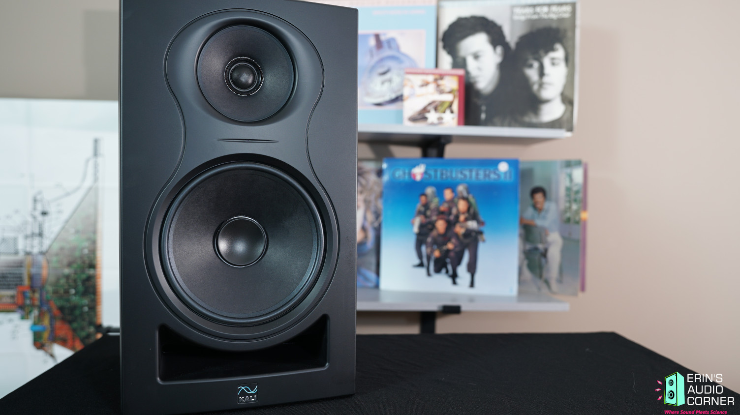
The Kali IN-8v2 is the second generation powered 3-way Studio Monitor featuring a 4-inch coaxial midrange/tweeter and an 8-inch midwoofer.

MSRP for the single speaker is approximately $399 USD and $800 USD for a pair.

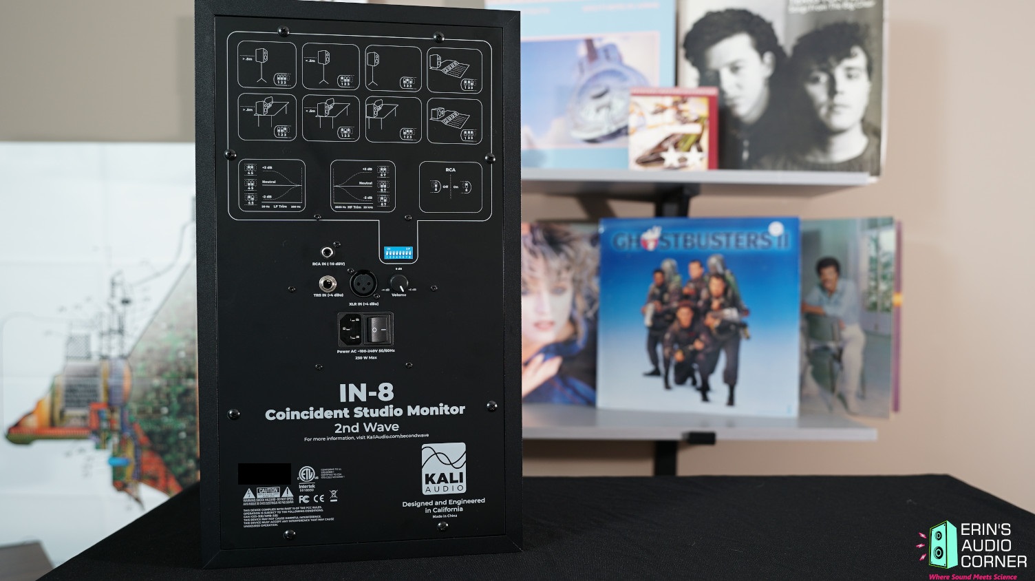
The back features a bank of dip switches for boundary settings (discussed later) and basic level adjustments. There is a volume knob and (3) input options: XLR, TRS and RCA phono.

CTA-2034 (SPINORAMA) and Accompanying Data

All data collected using Klippel’s Near-Field Scanner. The Near-Field-Scanner 3D (NFS) offers a fully automated acoustic measurement of direct sound radiated from the source under test. The radiated sound is determined in any desired distance and angle in the 3D space outside the scanning surface. Directivity, sound power, SPL response and many more key figures are obtained for any kind of loudspeaker and audio system in near field applications (e.g. studio monitors, mobile devices) as well as far field applications (e.g. professional audio systems). Utilizing a minimum of measurement points, a comprehensive data set is generated containing the loudspeaker’s high resolution, free field sound radiation in the near and far field. For a detailed explanation of how the NFS works and the science behind it, please watch the below discussion with designer Christian Bellmann:

The reference plane in this test is at the tweeter. Volume set to ‘0’ with XLR input. The dip switches were all set to ‘0’ for the free field setting.

Measurements are provided in a format in accordance with the Standard Method of Measurement for In-Home Loudspeakers (ANSI/CTA-2034-A R-2020). For more information, please see this link.

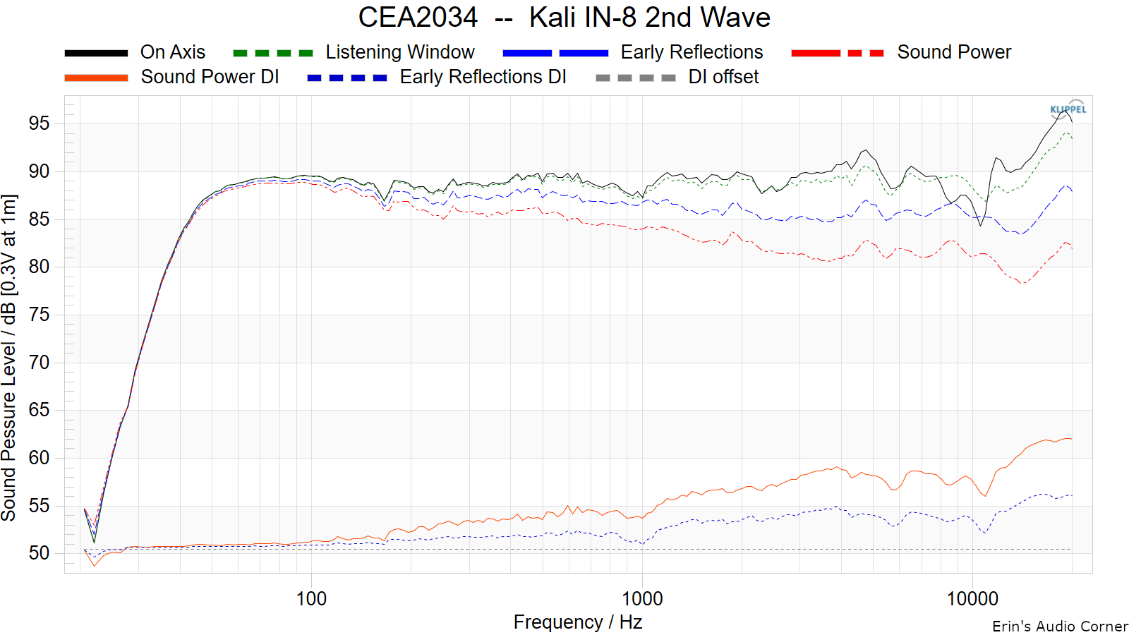
Note: The roll off rate of this speaker is sharp and therefore some noise was unavoidable at 25Hz which causes a spike in the response here. Ignore the response below 25Hz.

CTA-2034 / SPINORAMA:

The On-axis Frequency Response (0°) is the universal starting point and in many situations it is a fair representation of the first sound to arrive at a listener’s ears.

The Listening Window is a spatial average of the nine amplitude responses in the ±10º vertical and ±30º horizontal angular range. This encompasses those listeners who sit within a typical home theater audience, as well as those who disregard the normal rules when listening alone.

The Early Reflections curve is an estimate of all single-bounce, first-reflections, in a typical listening room.

Sound Power represents all the sounds arriving at the listening position after any number of reflections from any direction. It is the weighted rms average of all 70 measurements, with individual measurements weighted according to the portion of the spherical surface that they represent.

Sound Power Directivity Index (SPDI): In this standard the SPDI is defined as the difference between the listening window curve and the sound power curve.

Early Reflections Directivity Index (EPDI): is defined as the difference between the listening window curve and the early reflections curve. In small rooms, early reflections figure prominently in what is measured and heard in the room so this curve may provide insights into potential sound quality.

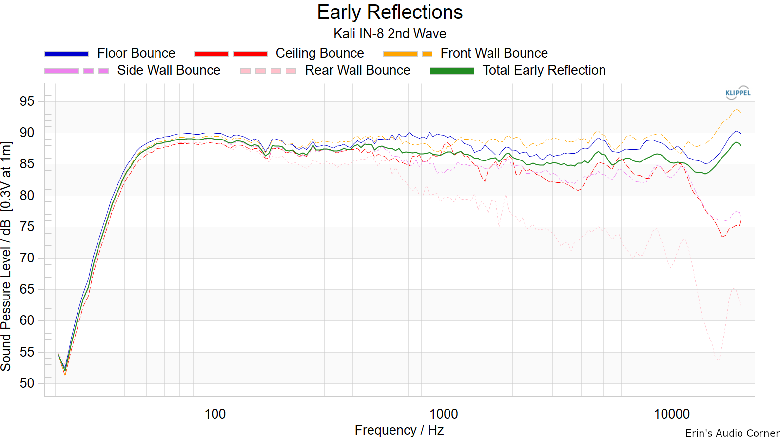
Early Reflections Breakout:

Floor bounce: average of 20º, 30º, 40º down

Ceiling bounce: average of 40º, 50º, 60º up

Front wall bounce: average of 0º, ± 10º, ± 20º, ± 30º horizontal

Side wall bounces: average of ± 40º, ± 50º, ± 60º, ± 70º, ± 80º horizontal

Rear wall bounces: average of 180º, ± 90º horizontal

Estimated In-Room Response:

In theory, with complete 360-degree anechoic data on a loudspeaker and sufficient acoustical and geometrical data on the listening room and its layout it would be possible to estimate with good precision what would be measured by an omnidirectional microphone located in the listening area of that room. By making some simplifying assumptions about the listening space, the data set described above permits a usefully accurate preview of how a given loudspeaker might perform in a typical domestic listening room. Obviously, there are no guarantees because individual rooms can be acoustically aberrant. Sometimes rooms are excessively reflective (“live”) as happens in certain hot, humid climates, with certain styles of interior décor and in under-furnished rooms. Sometimes rooms are excessively “dead” as in other styles of décor and in some custom home theaters where acoustical treatment has been used excessively. This form of post processing is offered only as an estimate of what might happen in a domestic living space with carpet on the floor and a “normal” amount of seating, drapes, and cabinetry.

For these limited circumstances it has been found that a usefully accurate Predicted In-Room (PIR) amplitude response, also known as a “room curve” is obtained by a weighted average consisting of 12 % listening window, 44 % early reflections and 44 % sound power. At very high frequencies errors can creep in because of excessive absorption, microphone directivity, and room geometry. These discrepancies are not considered to be of great importance.

Horizontal Frequency Response (0° to ±90°):

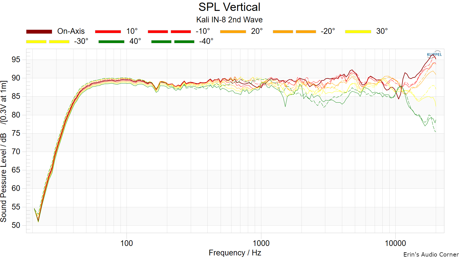
Vertical Frequency Response (0° to ±40°):

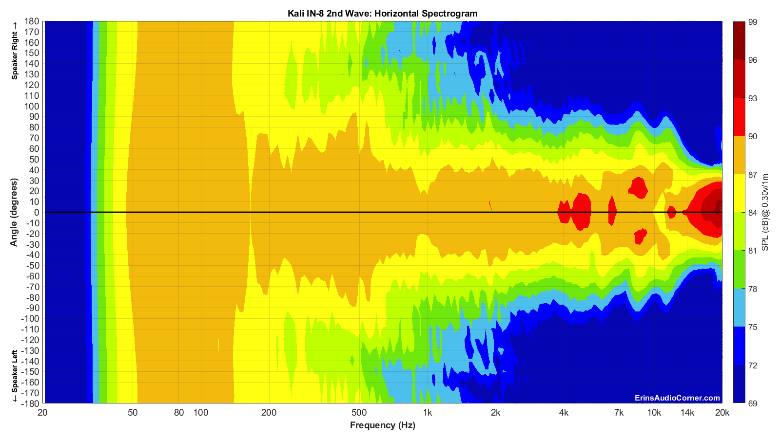
Horizontal Contour Plot (not normalized):

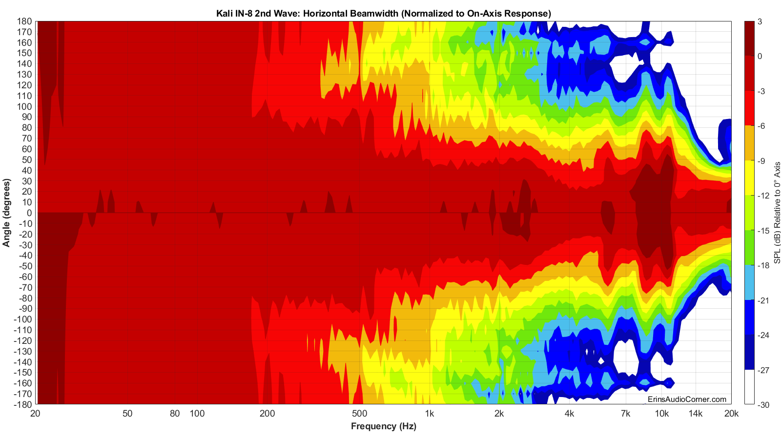
Horizontal Contour Plot (normalized):

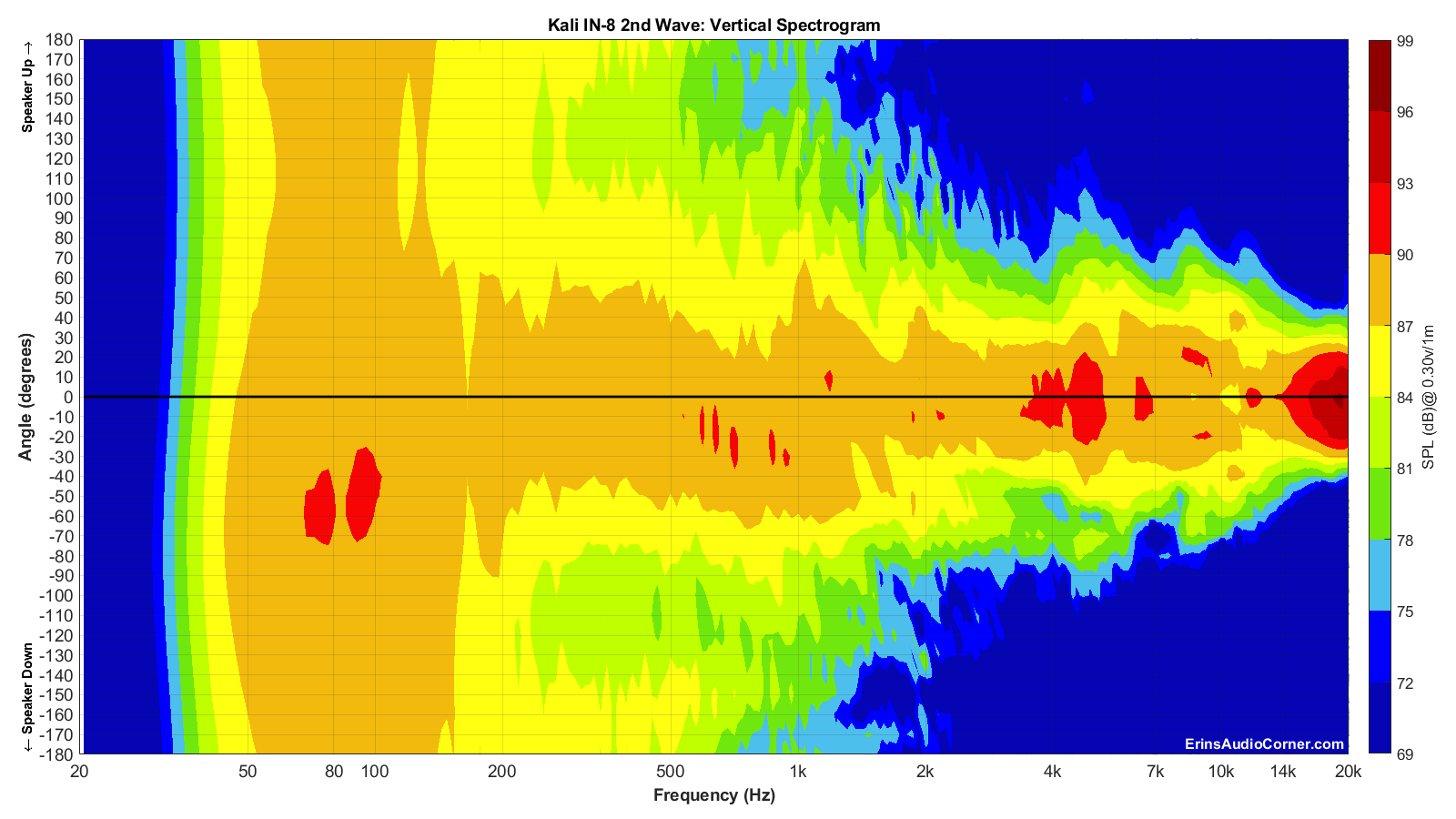
Vertical Contour Plot (not normalized):

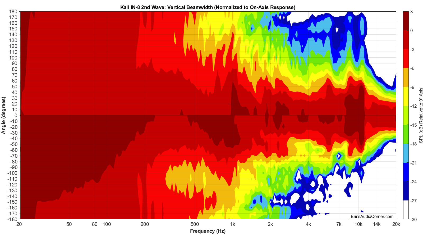
Vertical Contour Plot (normalized):

Additional Measurements

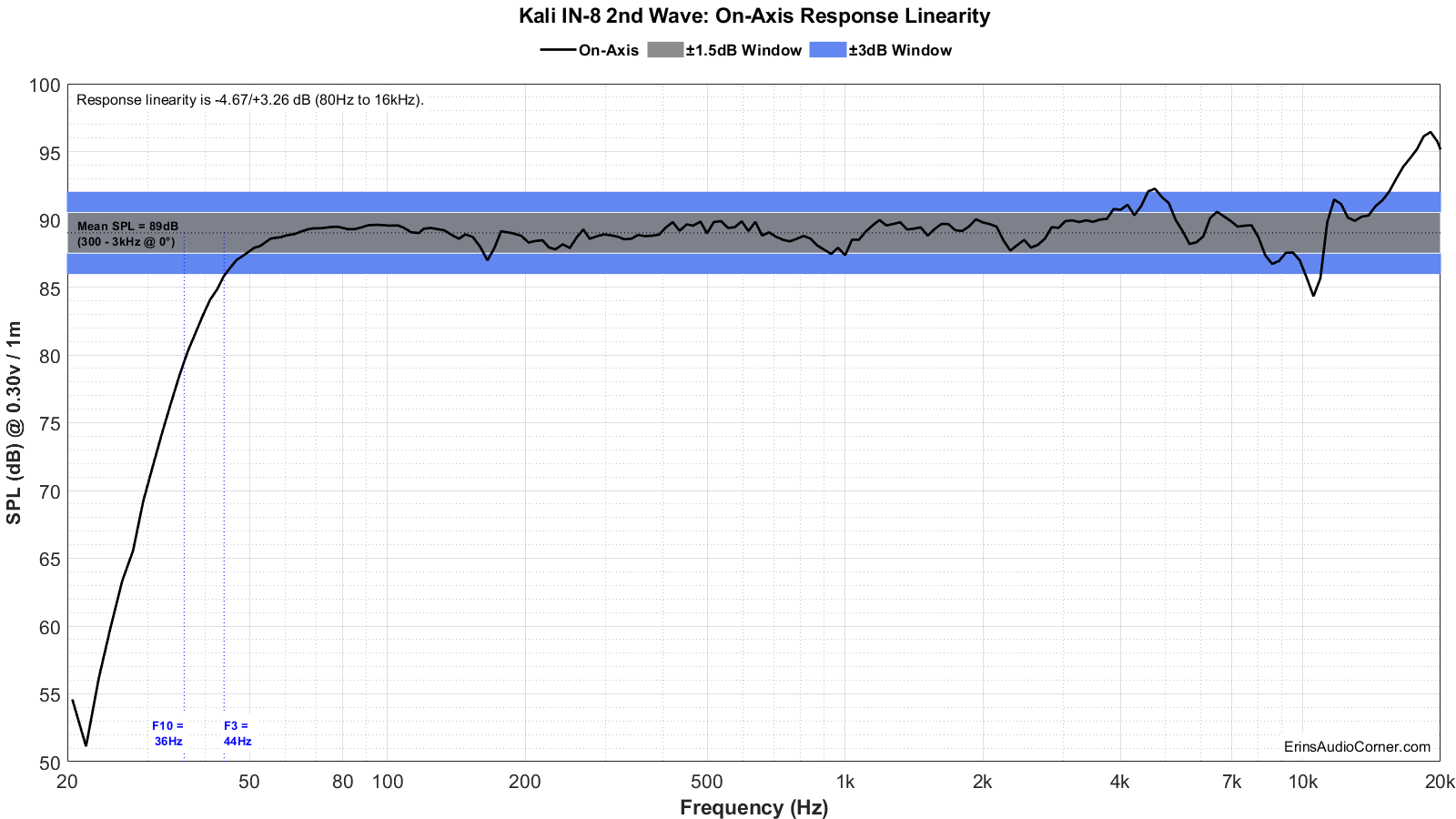
On-Axis Response Linearity

“Globe” Plots

These plots are generated from exporting the Klippel data to text files. I then process that data with my own MATLAB script to provide what you see. These are not part of any software packages and are unique to my tests.

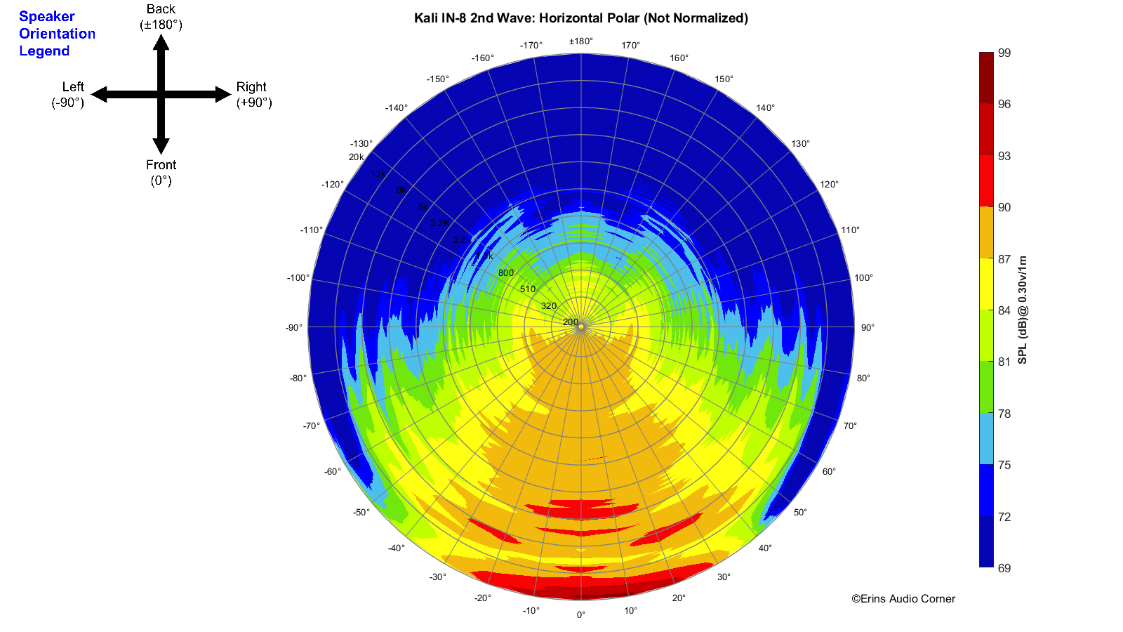
Horizontal Polar (Globe) Plot:
This represents the sound field at 2 meters - above 200Hz - per the legend in the upper left.

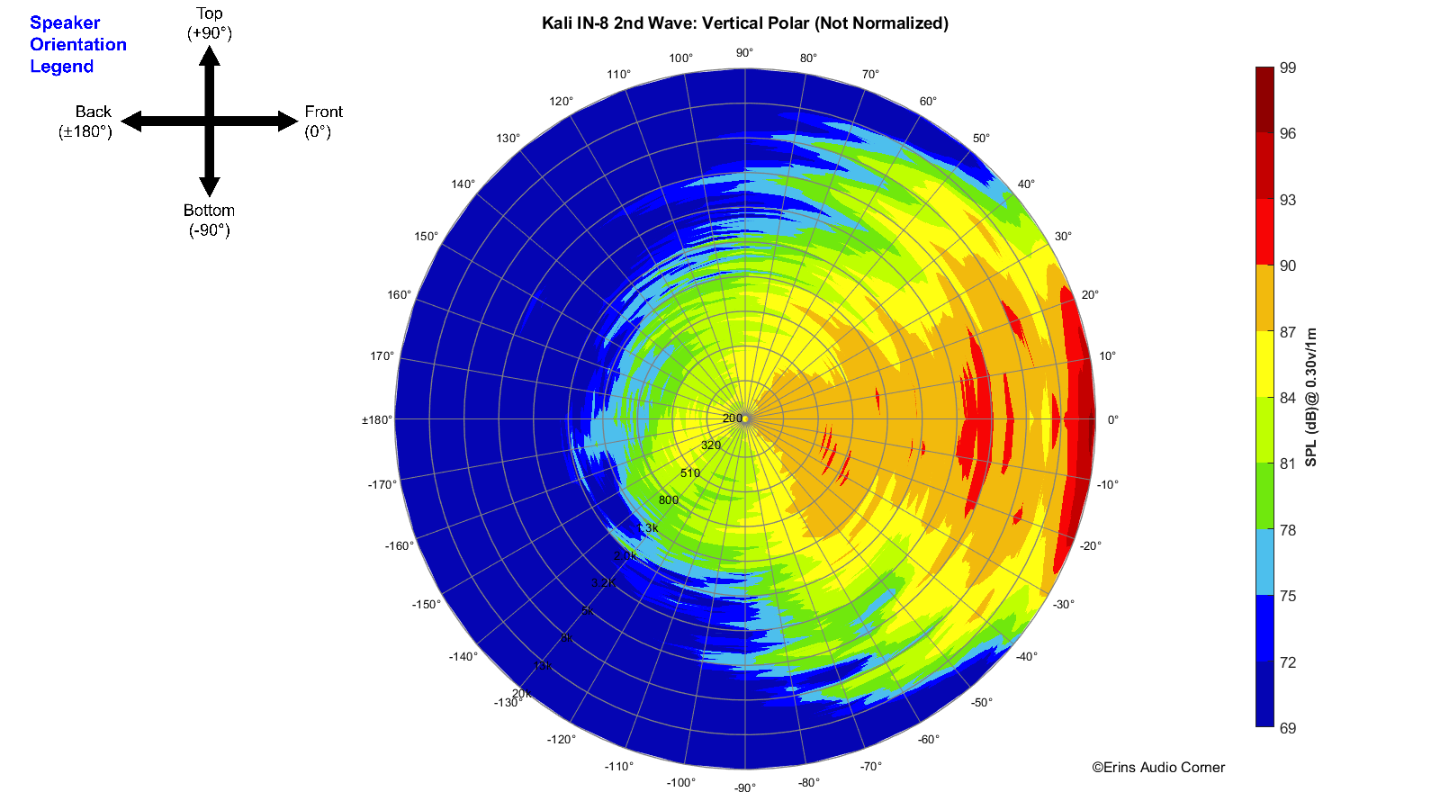
Vertical Polar (Globe) Plot:
This represents the sound field at 2 meters - above 200Hz - per the legend in the upper left.

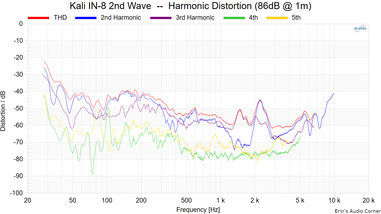
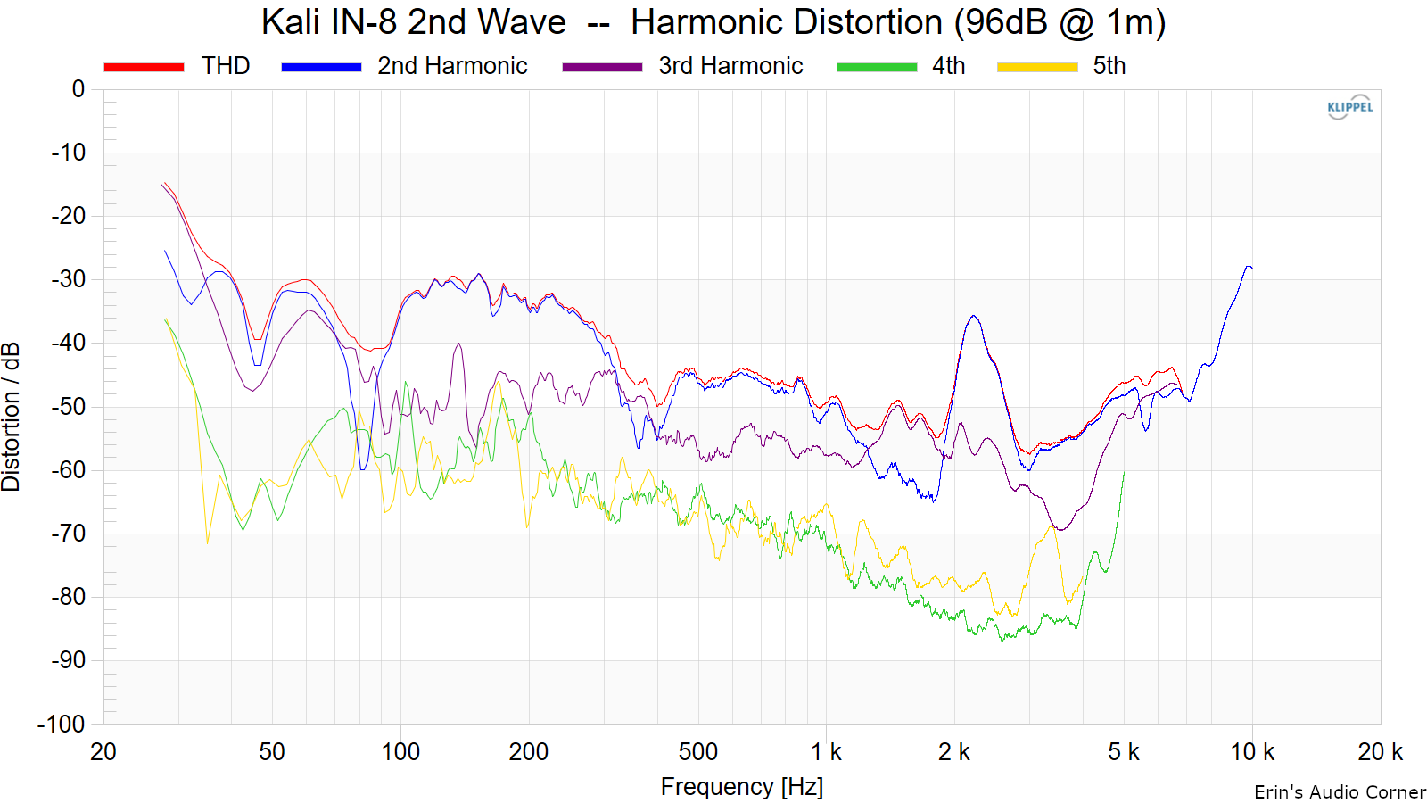
Harmonic Distortion

Harmonic Distortion at 86dB @ 1m:

Harmonic Distortion at 96dB @ 1m:

Dynamic Range (Instantaneous Compression Test)

The below graphic indicates just how much SPL is lost (compression) or gained (enhancement; usually due to distortion) when the speaker is played at higher output volumes instantly via a 2.7 second logarithmic sine sweep referenced to 76dB at 1 meter. The signals are played consecutively without any additional stimulus applied. Then normalized against the 76dB result.

The tests are conducted in this fashion:

1. 76dB at 1 meter (baseline; black)
2. 86dB at 1 meter (red)
3. 96dB at 1 meter (blue)
4. 102dB at 1 meter (purple)

The purpose of this test is to illustrate how much (if at all) the output changes as a speaker’s components temperature increases (i.e., voice coils, crossover components) instantaneously.

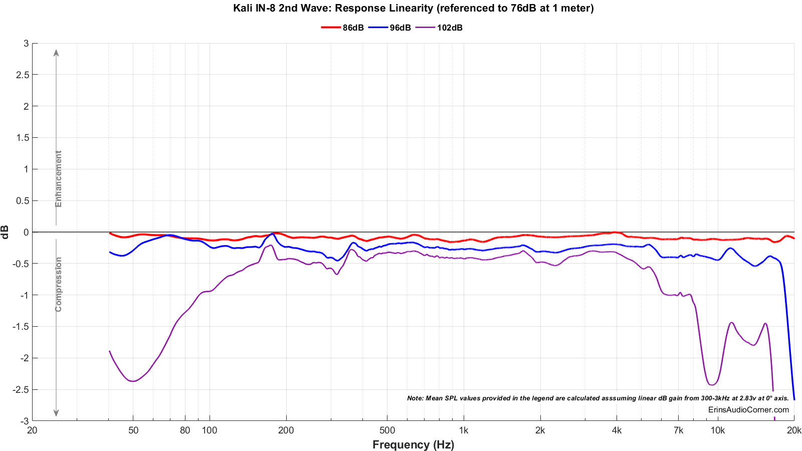
Based on my results above, it is obvious the output is limited (via internal DSP) somewhere above the 96dB @ 1m output level.

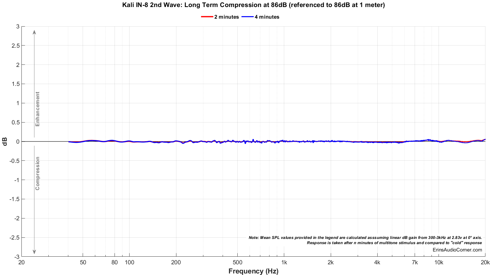
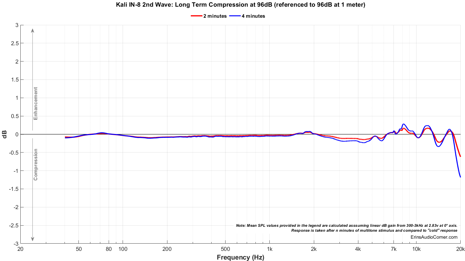
Long Term Compression Tests

The below graphics indicate how much SPL is lost or gained in the long-term as a speaker plays at the same output level for 2 minutes, in intervals. Each graphic represents a different SPL: 86dB and 96dB both at 1 meter.

The purpose of this test is to illustrate how much (if at all) the output changes as a speaker’s components temperature increases (i.e., voice coils, crossover components).

The tests are conducted in this fashion:

1. “Cold” logarithmic sine sweep (no stimulus applied beforehand)
2. Multitone stimulus played at desired SPL/distance for 2 minutes; intended to represent music signal
3. Interim logarithmic sine sweep (no stimulus applied beforehand) (Red in graphic)
4. Multitone stimulus played at desired SPL/distance for 2 minutes; intended to represent music signal
5. Final logarithmic sine sweep (no stimulus applied beforehand) (Blue in graphic)

The red and blue lines represent changes in the output compared to the initial “cold” test.

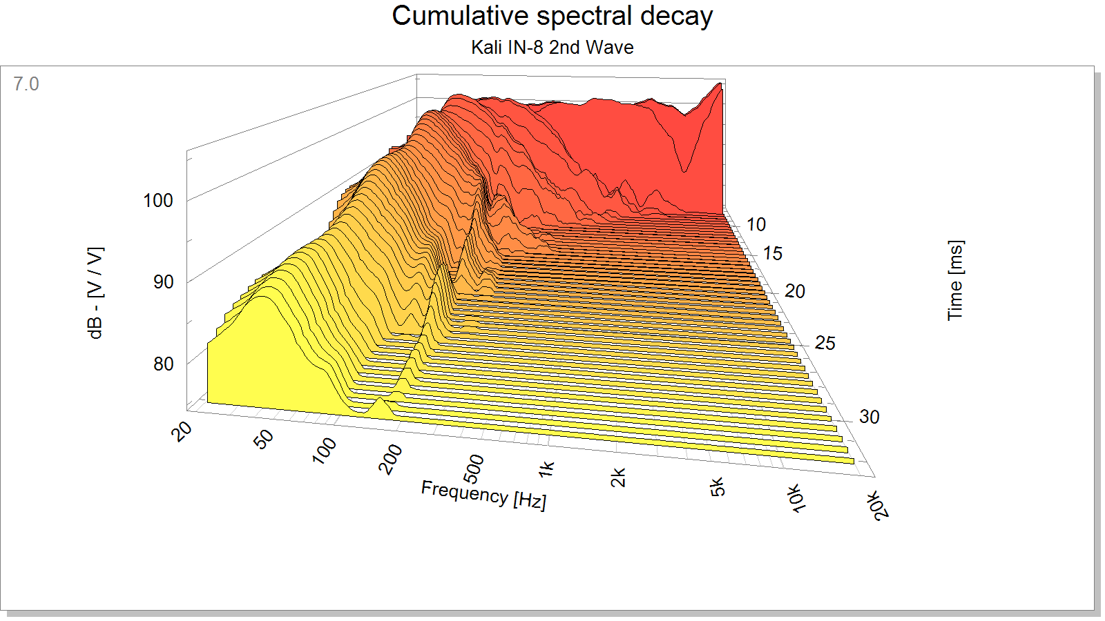
Cumulative Spectral Decay (CSD)

Boundary Settings

I tested this with the IN-5 and am providing it again here. I expect some bit of change from this model but likely not much (and possibly, not at all).

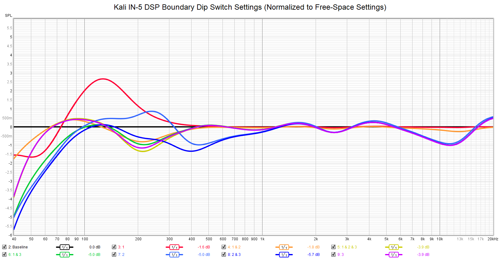
These speakers come with a set of pre-configured boundary settings that can be enabled easily via the dip switches on the back. Below is a close shot of the dip switches.

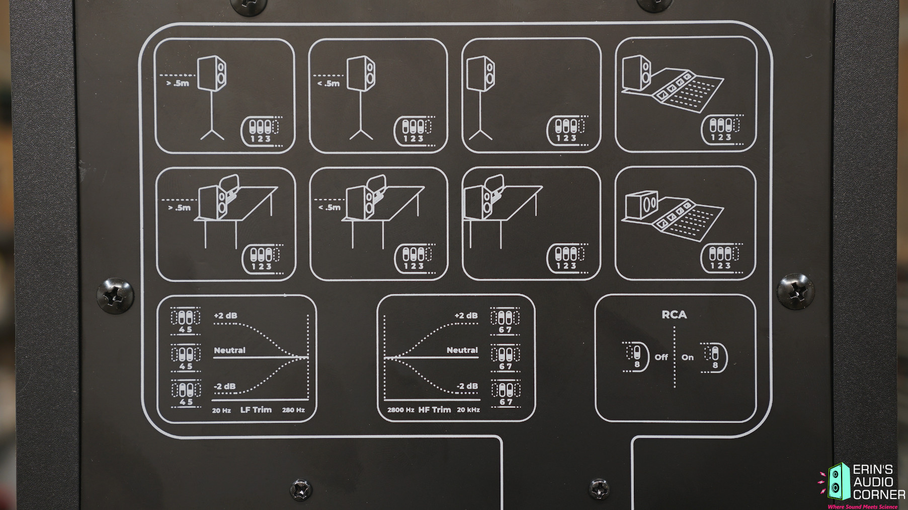
The dip switch combinations displayed above are labeled and plotted in the graphic below.

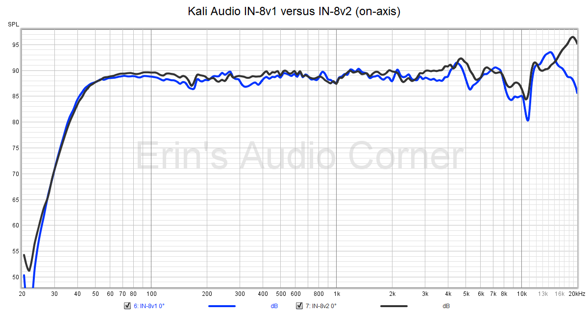
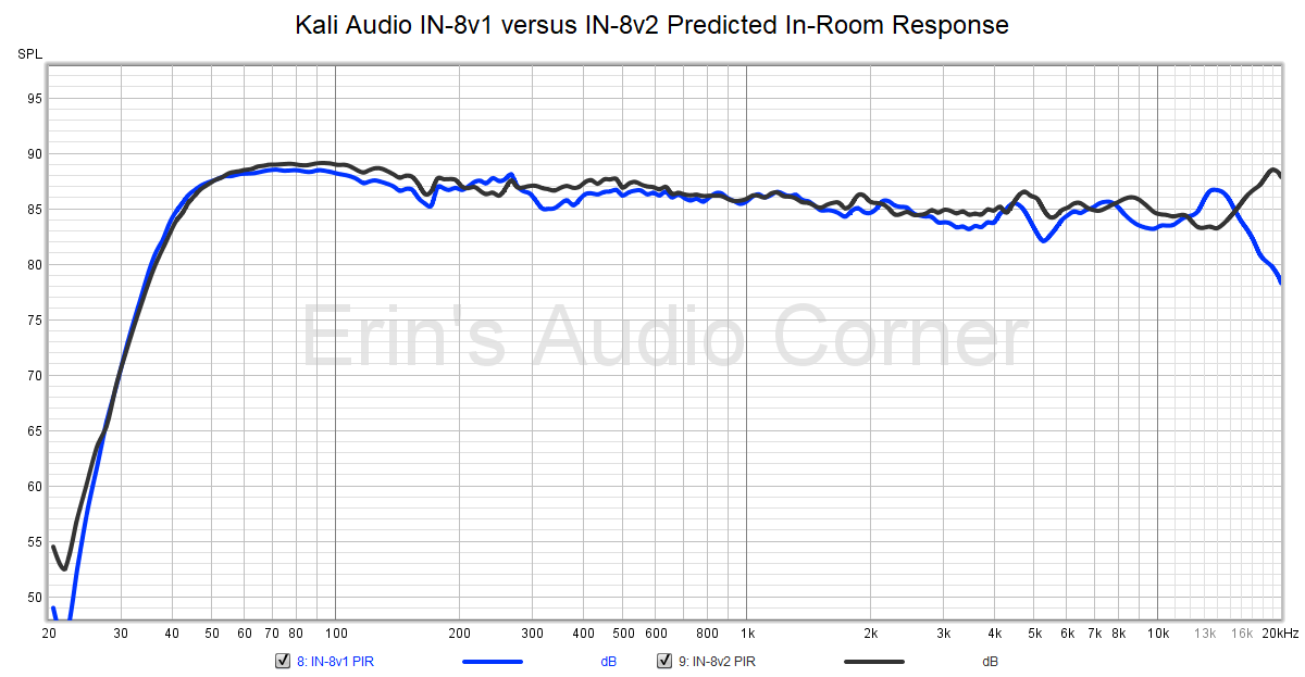
Comparison Against the Kali IN-8v1

• Blue = IN-8v1
• Black = IN-8v2

On-Axis Response:

Estimated In-Room Response:

Parting / Random Thoughts

If you want to see the music I use for evaluating speakers subjectively, see my Spotify playlist.

• Subjective listening was primarily at 1.5 meters but varied from 1 to 3 meters. Subjective listening was conducted at 80-95dB at this distance. Higher volumes were done simply to test the output capability in case one wants to try to sit further away.
• The front port means you have more ability to move these speakers in to the prime spot for your needs. And thanks to the dip switches you have more ability to place the speakers where you need; whether free standing, near a wall or on a console.
• The on-axis response isn’t flat but that’s the nature of coincident drivers. You’ll need to be off-axis a bit. Kali recommends 10°. My data jives with this, though, I would also recommend trying them off-axis by about 20°. Your mileage may vary. Just do not make the mistake of EQ’ing the on-axis response as this only alters the character of the sound in a negative way.
• There is zero mechanical noise from these speakers (pops, over-excursion, vent noise) even at higher volumes. However, these are intended to be used as nearfield monitors in the 1-2 meter range. Going past this will naturally mean you’ll need more volume and if you are listening at absurd levels, you will certainly run in to the built-in limiter throttling the output as I showed in my linearity test.
• There were only a couple of instances where I felt improvement was needed. One example was namely in the 4-5kHz region where - with some music (Lido Shuffle by Boz Skaggs, for example - the sound may jump out at you a bit, having a bit of “bite”. Using my EQ, I padded this down about 2dB and it really made a noticeable improvement. I think 1-2dB cut at 4.5kHz with even a graphic equalizer would make this a more pleasing speaker to most. More than 2dB takes the “edge” off instruments which dulls the sound.
• Another area that occasionally stood out to me was in the 100-200Hz where some lower vocals tended to sound a bit “hot”. It was a rare occurrence but noticeable, nonetheless. I took the speaker back out to the garage and measured it for CSD (provided previously). The CSD indicates a lingering resonance at roughly 160Hz. It is interesting to note there is a dip in the SPINORAMA data at this frequency but yet a peak in the dynamic compression test. Hmph.
• The bass is really nice and extends down to 50Hz easily. There are no bass boosts or issues in the bass region that call attention to themselves. Just neutral response that digs relatively deep.
• Hiss: Practically nonexistent. This is a very noticeable improvement over the IN-8v1.
• As for SPL levels, these are marketed as a near/mid-field speaker. My data shows the limiter kicking in somewhere above 96dB @ 1m. I had the output up to about 100dB at 1 meter to stress test with some Linkin Park and there were no mechanical issues that I could hear. I’d say that you could probably use these in the midfield in the lower 90’s pretty well but above that would be pushing it. Realistically, you shouldn’t be mixing music (or listening) above the 85dB range for long periods anyway. I do not know that I would recommend these for high volume listening more than 3 meters but for most volume levels and/or closer distances, a pair of these should be more than enough to satisfy your needs.

These are excellent speakers on a whole, to my ears. They are, in my opinion, an excellent value at the MSRP of only $800/pair. It is a great mixing/monitoring speaker and would do well in home audio applications (but be mindful of the output as the linearity changes at high output levels thanks to the built-in limiter). Frankly, I don’t know how Kali is able to produce such a nice speaker for such a reasonable price. I have no problem recommending the Kali IN-8 Second Wave.

In case you are wondering, no, Kali did not send me these speakers to review. They came from a viewer.

Support the Cause

If you like what you see here and want to help support the cause you might be interested in joining my Patreon, here. You can also contribute via PayPal (the big yellow button below).

Your support helps me pay for new items to test, hardware, miscellaneous items and costs of the site’s server space and bandwidth. All of which I otherwise pay out of pocket. So, if you can help chip in a few bucks, know that it is very much appreciated.

Alternatively, if you have a need to purchase anything through Amazon, please consider using my Amazon affiliate link below. It yields me a small commission at no additional cost to you and allows me to keep providing you with sweet data to make educated purchase decisions.

You can also join my Facebook and YouTube pages if you would like to follow along with updates.