Foreword / YouTube Video Review
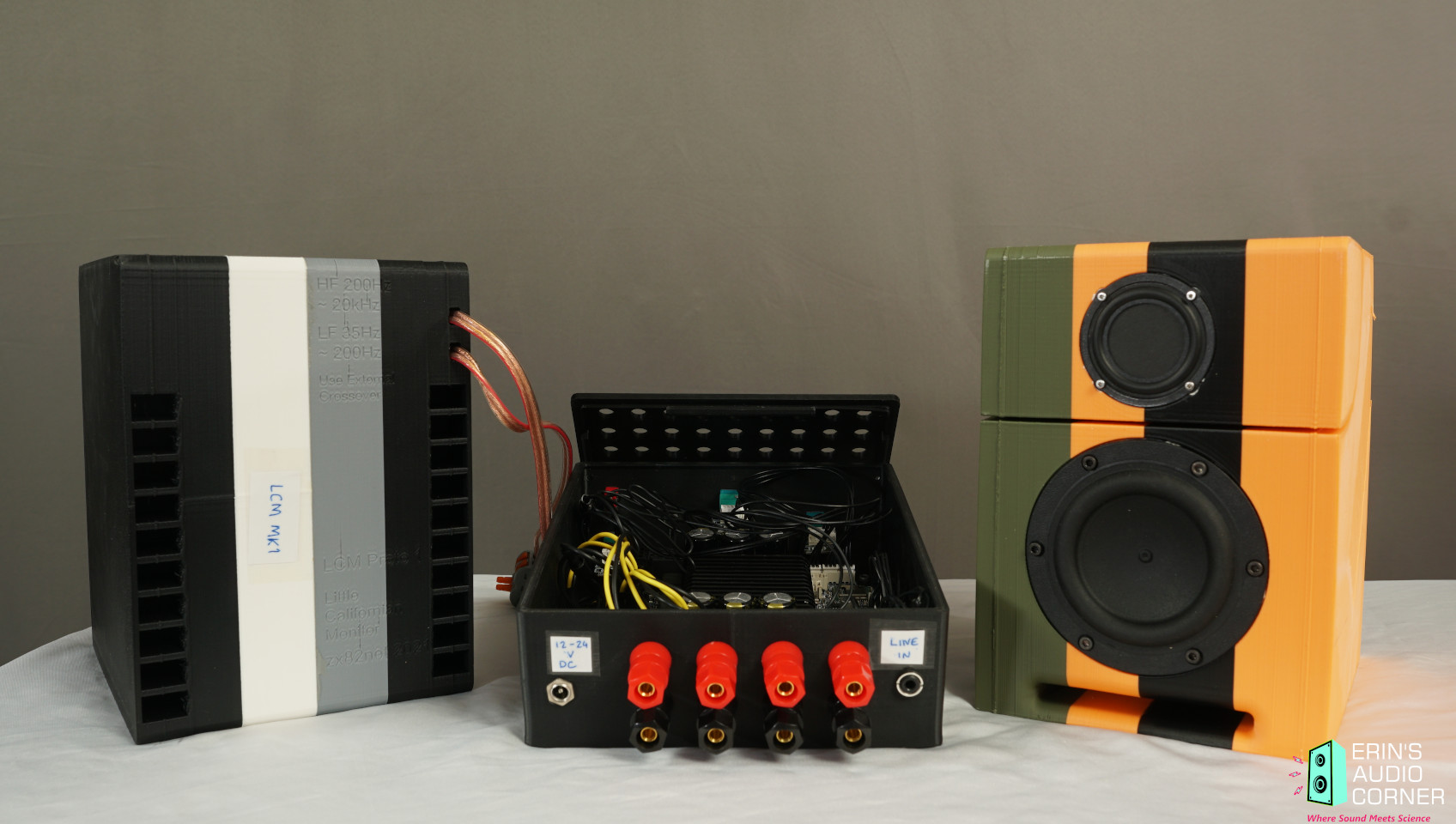
These speakers were loaned to me by their designer for review.
Also note the bottom section of this review will have some additional stuff that you might be interested in with respect to the DIY aspect of this speaker and verification of the completed speaker’s results.
The review on this website is a brief overview and summary of the objective performance of this speaker. It is not intended to be a deep dive. Moreso, this is information for those who prefer “just the facts” and prefer to have the data without the filler. The video below has more discussion.
Information and Photos
Specs from the manufacturer can be found here.
- 3-D Printed enclosure
- Tang Band W3 1876S 3" Subwoofer driver
- Tectonic TEBM35C10-4 2" BMR driver
- Features Dayton Audio KABD-4100 4x100w Amp+DSP
Short backstory here is: I saw this speaker on Instructables.com, thought it was neat, reached out to the designer and he sent them over for me to test out. These things are too cool for school. 3-D printed enclosure, active DSP + amp, small, decent linearity (that can and likely will be updated based on the data in this review) and overall just a neat little project.
It won’t knock your socks off with output, but it’ll surprise you and makes a fun little project that incorporates a lot of DIY capability from enclosure printing to DSP design using the Dayton amp/DSP which features Sigma Studio DSP.
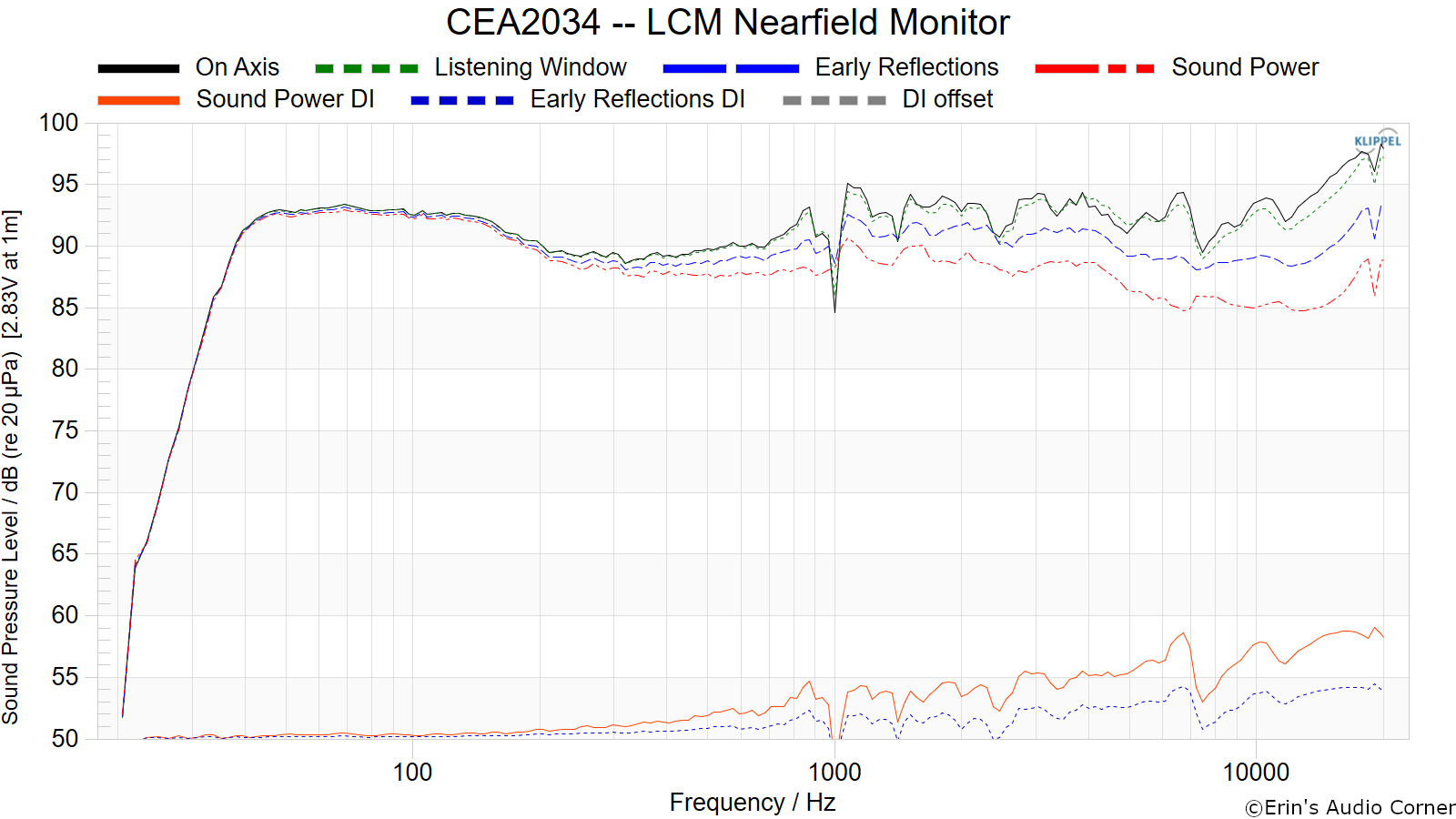
CTA-2034 (SPINORAMA) and Accompanying Data
All data collected using Klippel’s Near-Field Scanner. The Near-Field-Scanner 3D (NFS) offers a fully automated acoustic measurement of direct sound radiated from the source under test. The radiated sound is determined in any desired distance and angle in the 3D space outside the scanning surface. Directivity, sound power, SPL response and many more key figures are obtained for any kind of loudspeaker and audio system in near field applications (e.g. studio monitors, mobile devices) as well as far field applications (e.g. professional audio systems). Utilizing a minimum of measurement points, a comprehensive data set is generated containing the loudspeaker’s high resolution, free field sound radiation in the near and far field. For a detailed explanation of how the NFS works and the science behind it, please watch the below discussion with designer Christian Bellmann:
The reference plane in this test is at the mid/tweeter.
Measurements are provided in a format in accordance with the Standard Method of Measurement for In-Home Loudspeakers (ANSI/CTA-2034-A R-2020). For more information, please see this link.
CTA-2034 / SPINORAMA:
The On-axis Frequency Response (0°) is the universal starting point and in many situations it is a fair representation of the first sound to arrive at a listener’s ears.
The Listening Window is a spatial average of the nine amplitude responses in the ±10º vertical and ±30º horizontal angular range. This encompasses those listeners who sit within a typical home theater audience, as well as those who disregard the normal rules when listening alone.
The Early Reflections curve is an estimate of all single-bounce, first-reflections, in a typical listening room.
Sound Power represents all of the sounds arriving at the listening position after any number of reflections from any direction. It is the weighted rms average of all 70 measurements, with individual measurements weighted according to the portion of the spherical surface that they represent.
Sound Power Directivity Index (SPDI): In this standard the SPDI is defined as the difference between the listening window curve and the sound power curve.
Early Reflections Directivity Index (EPDI): is defined as the difference between the listening window curve and the early reflections curve. In small rooms, early reflections figure prominently in what is measured and heard in the room so this curve may provide insights into potential sound quality.
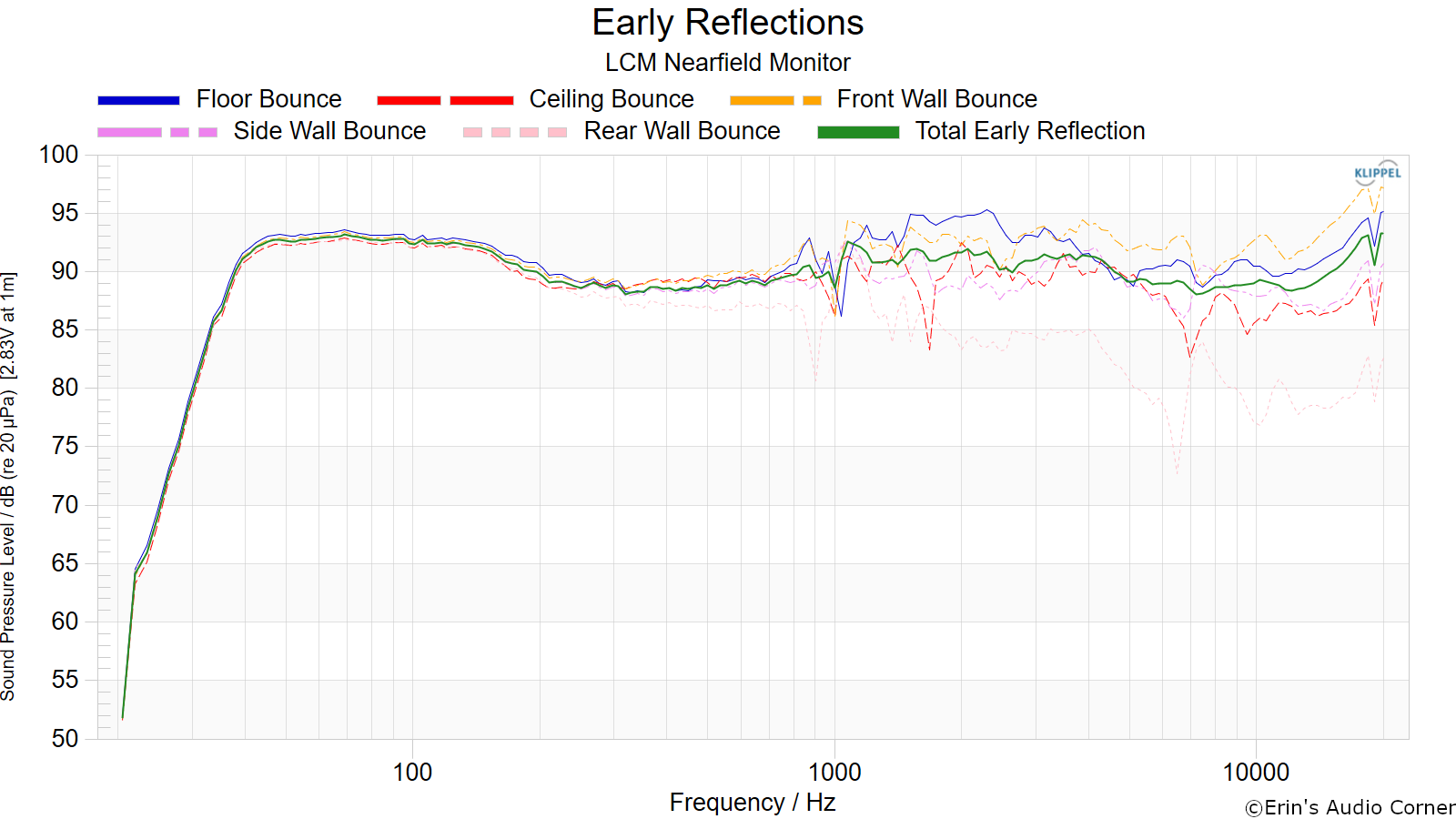
Early Reflections Breakout:
Floor bounce: average of 20º, 30º, 40º down
Ceiling bounce: average of 40º, 50º, 60º up
Front wall bounce: average of 0º, ± 10º, ± 20º, ± 30º horizontal
Side wall bounces: average of ± 40º, ± 50º, ± 60º, ± 70º, ± 80º horizontal
Rear wall bounces: average of 180º, ± 90º horizontal
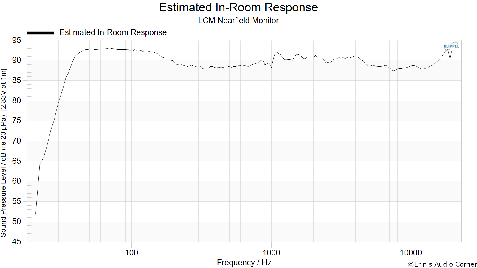
Estimated In-Room Response:
In theory, with complete 360-degree anechoic data on a loudspeaker and sufficient acoustical and geometrical data on the listening room and its layout it would be possible to estimate with good precision what would be measured by an omnidirectional microphone located in the listening area of that room. By making some simplifying assumptions about the listening space, the data set described above permits a usefully accurate preview of how a given loudspeaker might perform in a typical domestic listening room. Obviously, there are no guarantees, because individual rooms can be acoustically aberrant. Sometimes rooms are excessively reflective (“live”) as happens in certain hot, humid climates, with certain styles of interior décor and in under-furnished rooms. Sometimes rooms are excessively “dead” as in other styles of décor and in some custom home theaters where acoustical treatment has been used excessively. This form of post processing is offered only as an estimate of what might happen in a domestic living space with carpet on the floor and a “normal” amount of seating, drapes and cabinetry.
For these limited circumstances it has been found that a usefully accurate Predicted In-Room (PIR) amplitude response, also known as a “room curve” is obtained by a weighted average consisting of 12 % listening window, 44 % early reflections and 44 % sound power. At very high frequencies errors can creep in because of excessive absorption, microphone directivity, and room geometry. These discrepancies are not considered to be of great importance.
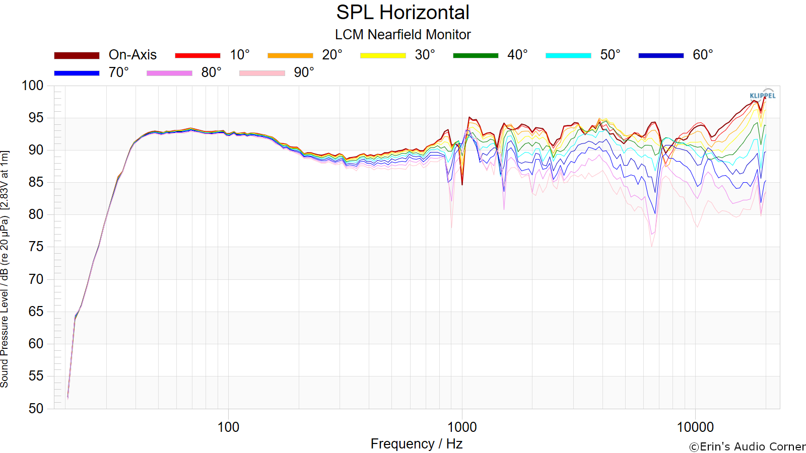
Horizontal Frequency Response (0° to ±90°):
Vertical Frequency Response (0° to ±40°):

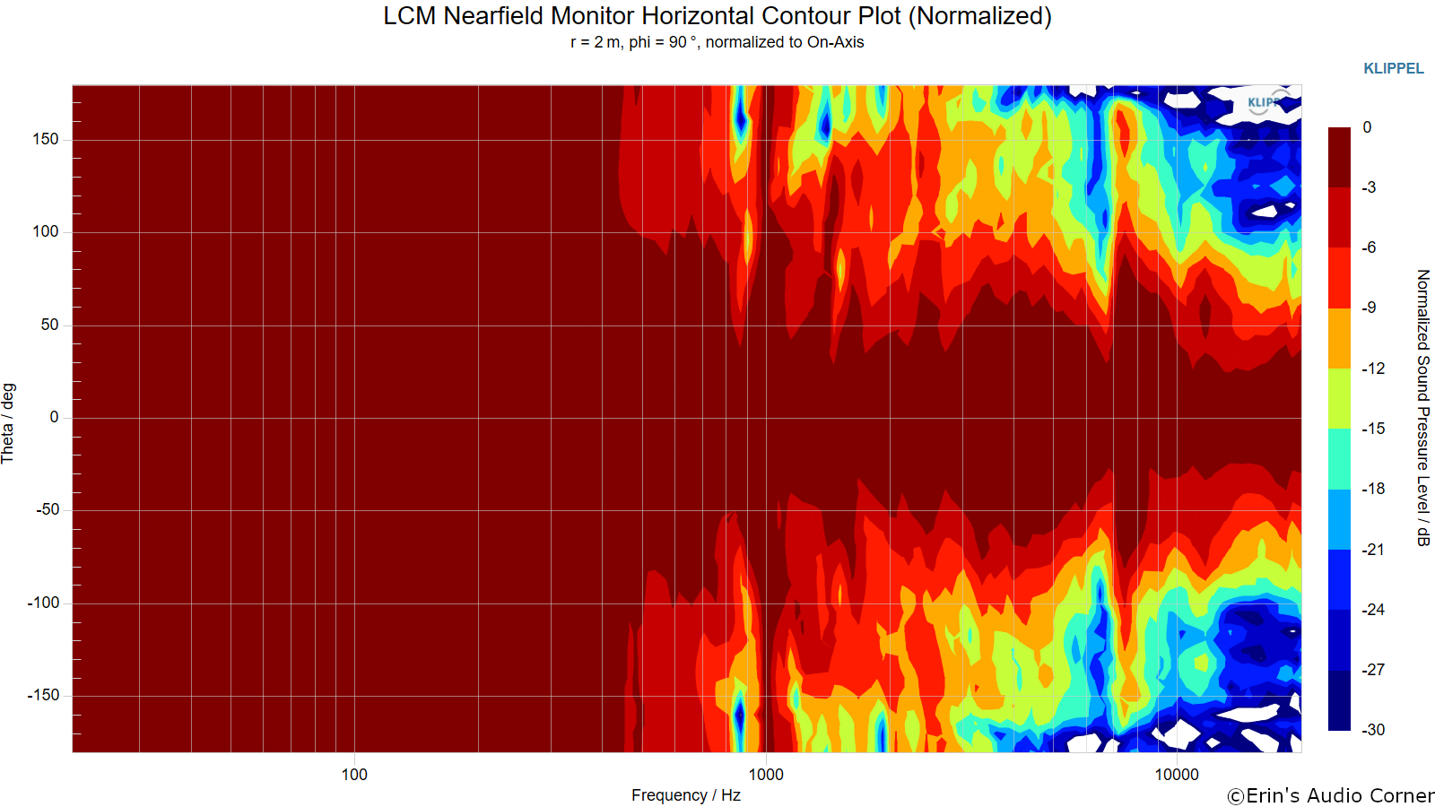
Horizontal Contour Plot (normalized):
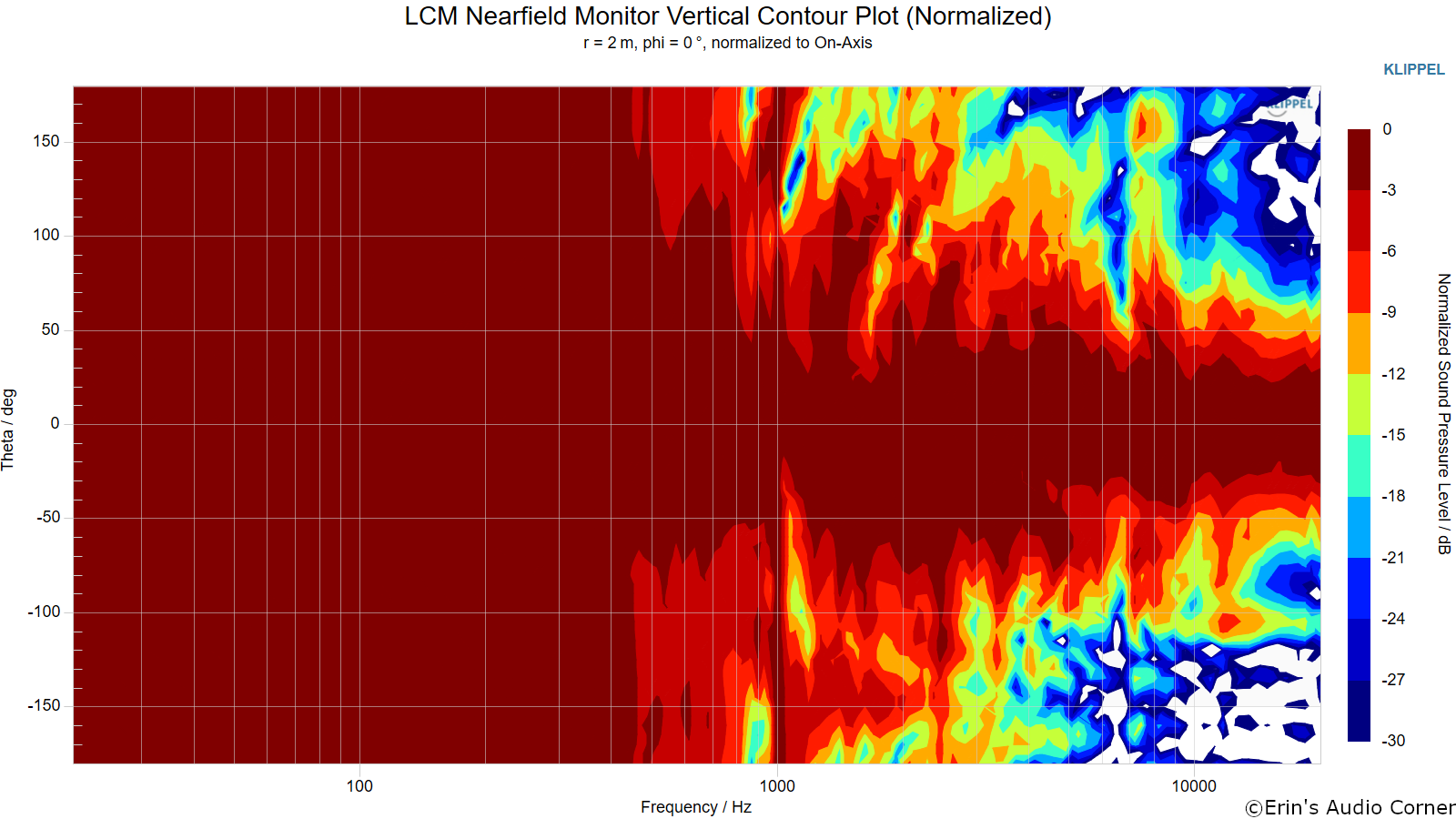
Vertical Contour Plot (normalized):
“Globe” Plots
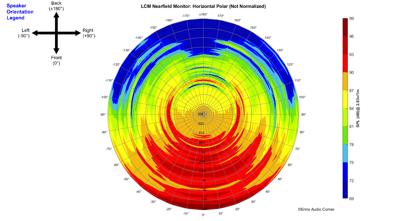
Horizontal Polar (Globe) Plot:
This represents the sound field at 2 meters - above 200Hz - per the legend in the upper left.
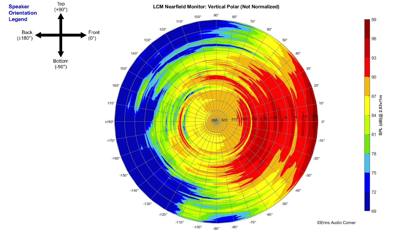
Vertical Polar (Globe) Plot:
This represents the sound field at 2 meters - above 200Hz - per the legend in the upper left.
Additional Measurements
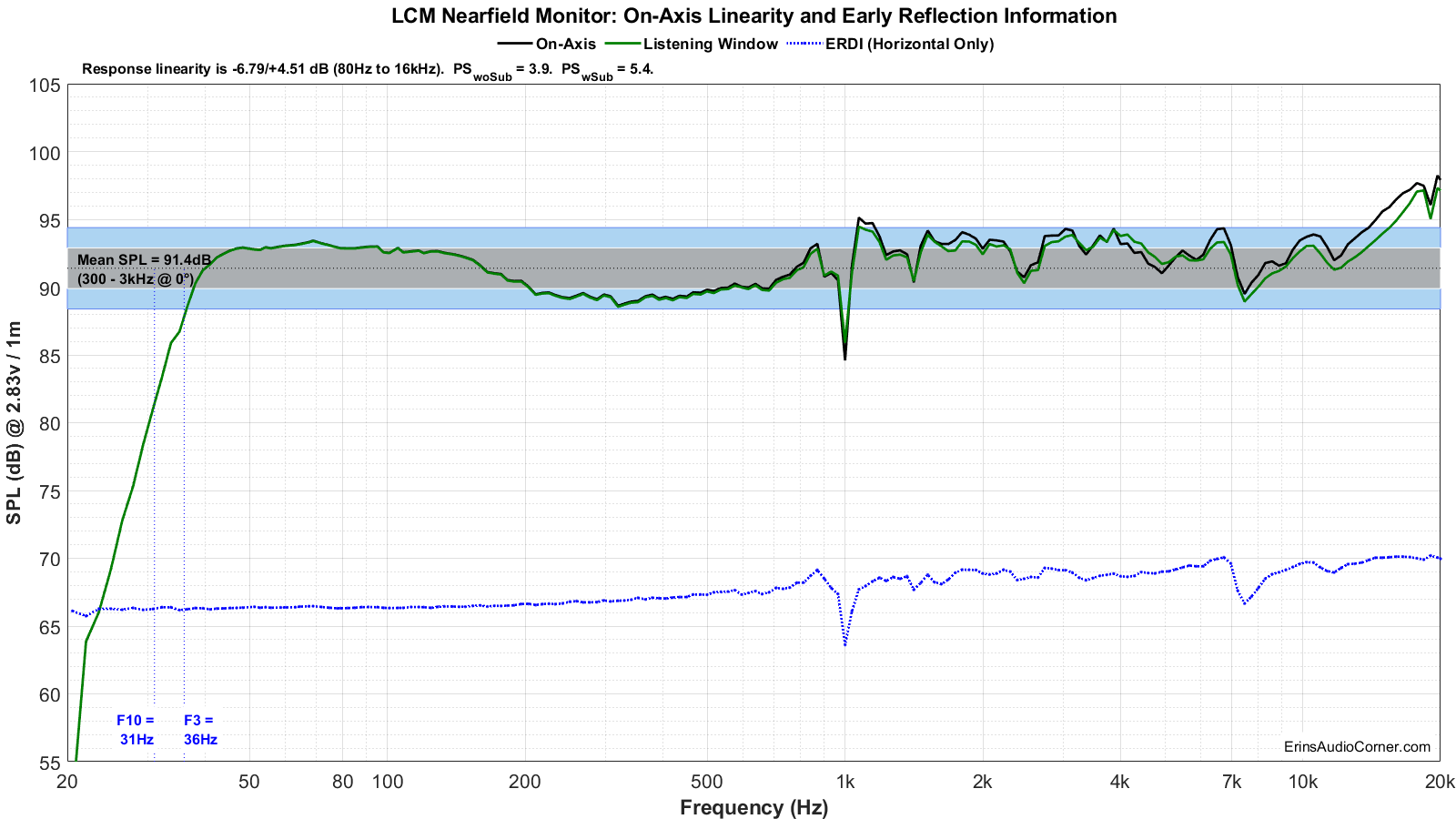
Response Linearity
Impedance Magnitude and Phase
N/A
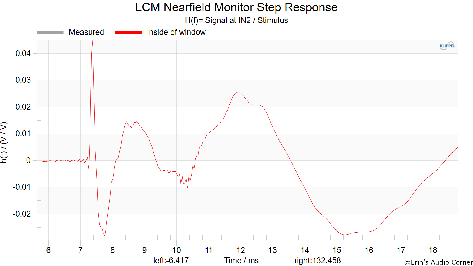
Step Response
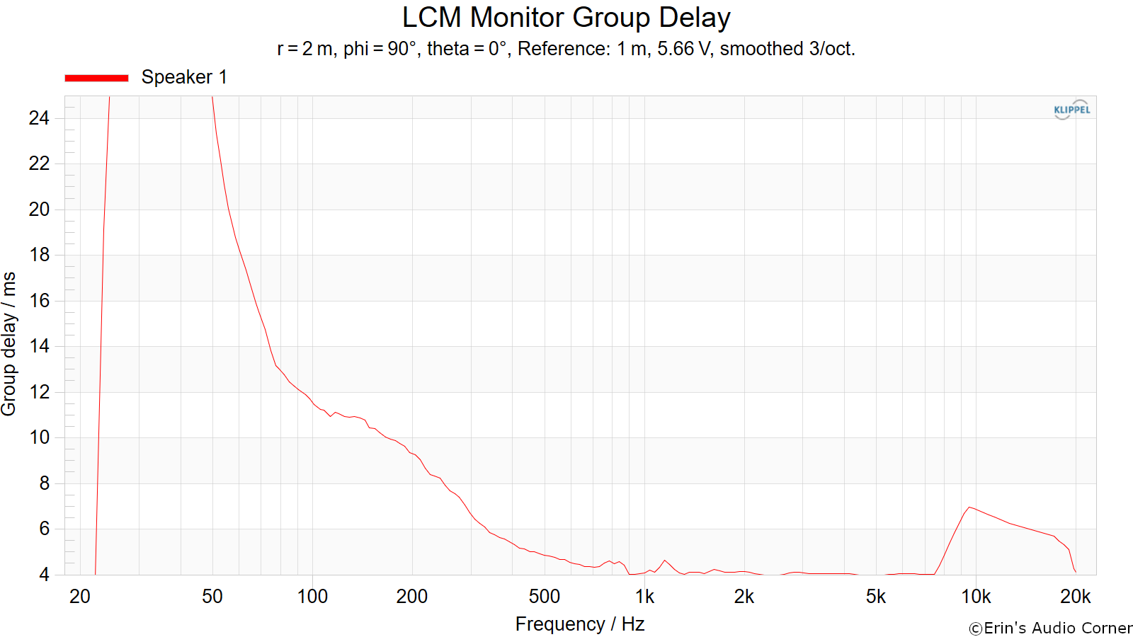
Group Delay
Harmonic Distortion
Harmonic Distortion at 86dB @ 1m:
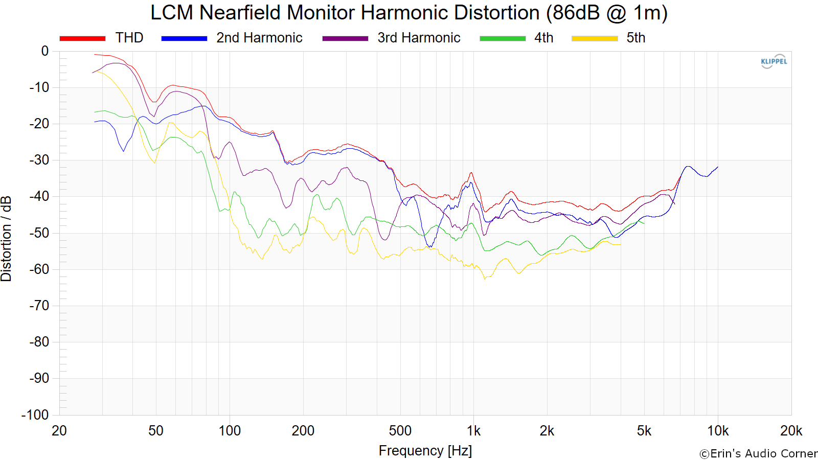
Max Speaker output is about 90dB or so. I couldn’t do a 96dB distortion test.
Dynamic Range (Instantaneous Compression Test)
Max output is about 90dB/1m. Therefore, the compression test was pretty much useless as I could only test 86dB against 76dB.
Parting / Random Thoughts
As stated in the Foreword, this written review is purposely a cliff’s notes version. For details about the performance (objectively and subjectively) please watch the YouTube video. But a couple quick notes based on my listening and what I see in the data:
- Neat project. Never seen anything like it before and all the instructions to build it are available for free on the instructables website.
- Decent linearity that would only take a minor EQ adjustment in the midrange to flatten the response (which the designer has told me he will try to implement).
- High volumes result in very audible resonances and distortion around 200hz so these really are limited-use in nearfield applications.
Contribute / Support
If you find this review helpful and want to help support the cause there are a few ways you can do so below. Your support helps me pay for new items to test, hardware, miscellaneous items needed for testing and costs of the site’s server space and bandwidth. Any help is very much appreciated.
Join my Patreon: Become a Patron!
Or using my product affiliate link below to buy this speaker or anything they sell that you want to try out. This will earn me a small commission at no additional cost to you. You can use these links anytime, now or in the future.
You can also join my Facebook and YouTube pages if you’d like to follow along with updates.