YouTube Review link
If you want help understanding what this data means, watch the video below.
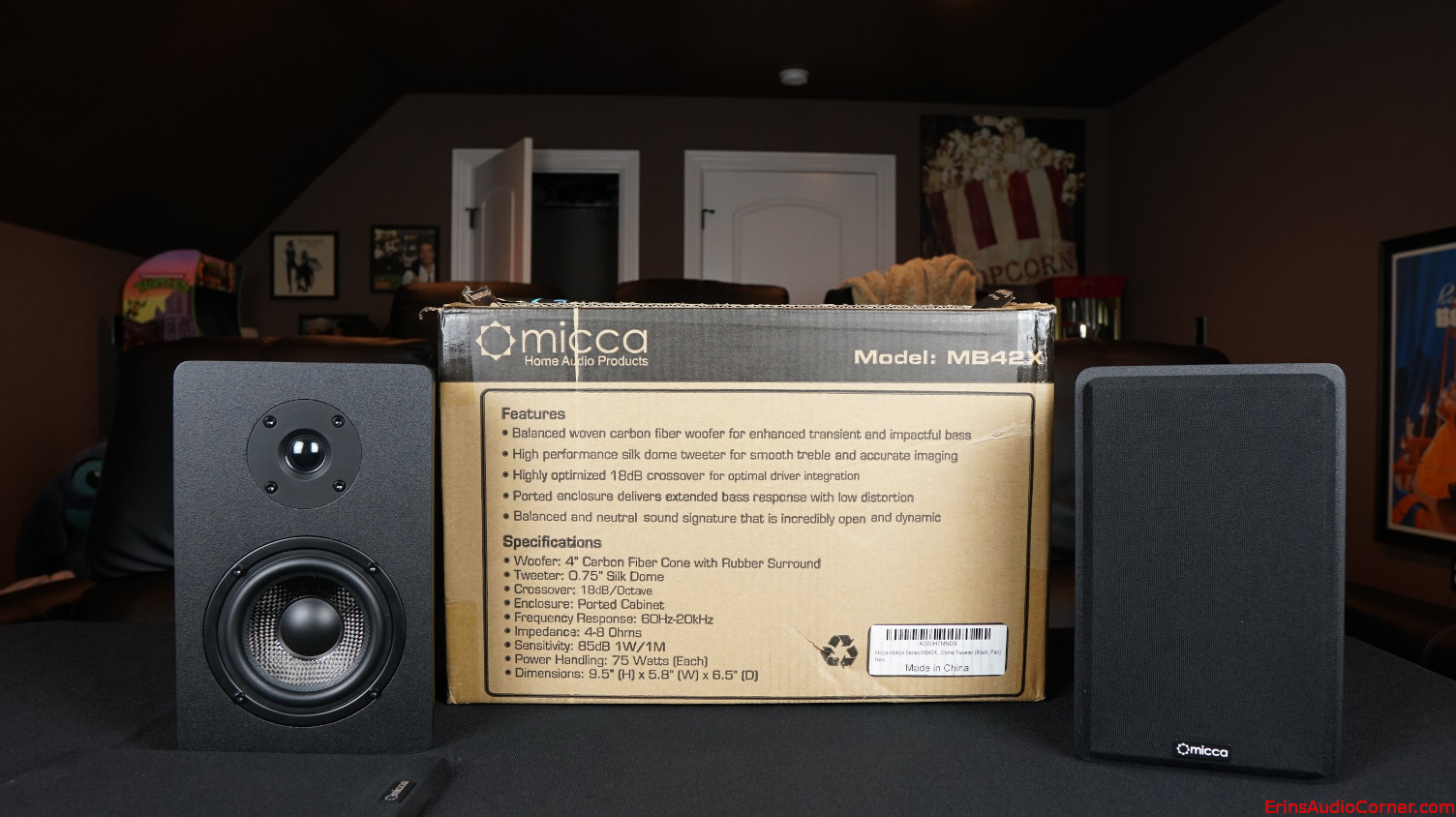
Intro, Product Specs and Photos
I purchased this speaker to compare against my recently reviewed Neumi BS5 (link here). This speaker is quite a bit smaller than the Neumi, which I discuss in my video above, but I was optimistic about its performance based on many other past reviewers’ positive impressions. Unfortunately, my listening session resulted in me turning off the speakers about 7 tracks in to it and I walked away rather disgusted. When I later tested the speaker and looked at the objective data, I realized why I hated their sound. The response curve of the Micca MB42X MKIII is extremely non-linear; exhibiting as a wholly recessed midrange, a prominent bump between 1-2kHz and poor linearity above 4kHz. The distortion is high. The compression is high. There’s truly nothing positive I can say about this speaker. I even went so far as to use my Dayton DATs to sweep both speakers to make sure the impedance curves matched because I thought maybe one of them was damaged but that wasn’t the case.
It is no surprise this speaker does not get my recommendation. At any rate, if, after you read this review, you still want to purchase a set, you can help the site by purchasing through the link below which earns me a small commission.
Though, I suggest you buy the Neumi BS5 if you are in the market for a sub-$100 bookshelf speaker. The Neumi is the same price as these Micca speakers and the Neumi performance is leagues better than the Micca. Here’s a link to the Neumi BS5:
Now, let’s get to the data so you can see why I heard what I heard.
Objective Data
Foreword: Subjective Analysis vs Objective Data (click for more)
If you have seen my past reviews, you know that I am of the mindset that objective data is at least as important as someone's subjective evaluation of a speaker. If not more. Why? Because every room is different. Every listener is different. Some know what to listen for. Others know what they want to hear based on their own preference (i.e., some prefer extended bass, some prefer more midbass punch between 120-150Hz, some prefer a response with a dip around 4kHz, etc., etc.). What one person wants or expects may be opposite of another. Additionally, the room will impact the performance and therefore what the listener hears. This means when you read another's subjective-only review you are left to resolve those variables on your own. That's not likely to happen. Unless there is objective data you can use to get an idea of the performance. With objective data you can begin to understand why the subjective review turned out the way it did. Notably, objective data keeps reviewers honest. It's hard for a reviewer to legitimately bash one product but elevate another when the two measure practically the same in every regard. Not to say two similarly measuring speakers cannot subjectively sound different. Though, odds are if they do measure the same then a huge subjective difference is most likely attributed to other issues such as setup conditions, bias, etc. Objective data is the key to accountability. Simply put: if the measurements are taken with care and you understand them, you can rely on data to help paint a more accurate description of performance than a few adjectives from your favorite reviewer (myself included). As you will see, objective measurements can provide a lot of insight in to how the speaker will perform in your room.However, when possible, it is always best to demo speakers in your own room. Not simply because of subjective performance. But because of other factors such as aesthetics, pride of ownership, etc. In my experience, all these factors play in to how the listener “connects” with the system. A good shop or manufacturer understands this and allows buyers to try items out at home before purchasing or they offer a reasonable return policy. If you question the performance and can demo the speakers in your own home, I suggest you take advantage of the opportunity.
For all the reasons listed above: What I provide here is objective-heavy analysis. I still provide my own subjective experience but with in-room measurements at my listening position(s) so we can understand why I heard what I heard. Is it the room, the actual speaker itself, my brain, or a combination?
Now that you understand my motives, let’s get started with the review.
Unless otherwise noted, all the data below was captured using Klippel Distortion Analyzer 2 and Klippel modules (TRF, DIS, LPM, ISC to name a few). Most of the data was exported to a text file and then graphed using my own MATLAB scripts in order to present the data in a specific way I prefer. However, some is given using Klippel’s graphing.
Impedance Phase and Magnitude:
Impedance measurements are provided both at 0.10 volts RMS and 2.83 volts RMS. The low-level voltage version is standard because it ensures the speaker/driver is in linear operating range. The higher voltage is to see what happens when the output voltage is increased to the 2.83vRMS speaker sensitivity test.
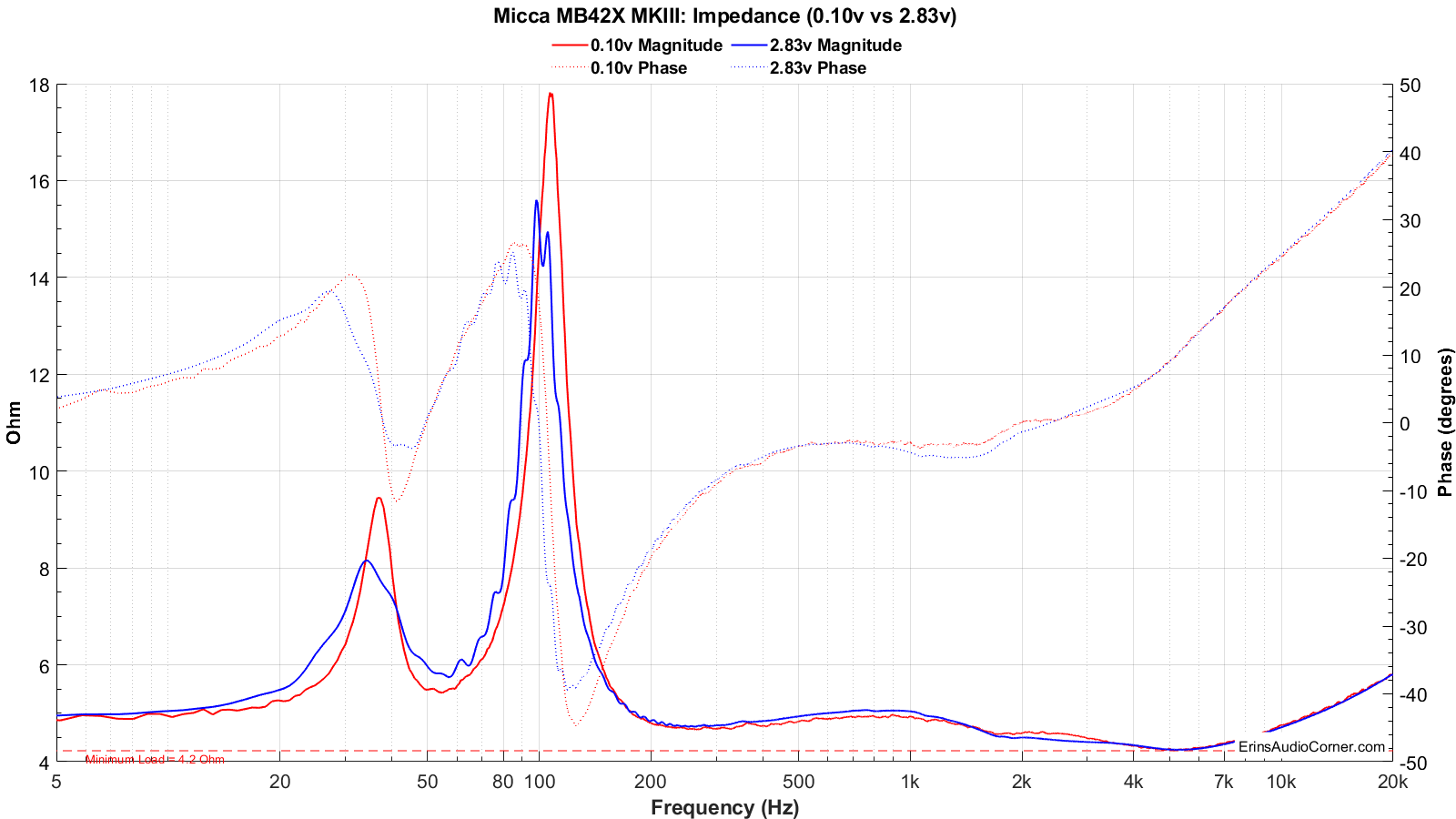
From the above data we can see the following:
- The tuning frequency of the enclosure is approximately 50Hz.
- The minimum impedance dips to about 4.2 Ohms around 1.4kHz with a nominal impedance at about 5 Ohms.
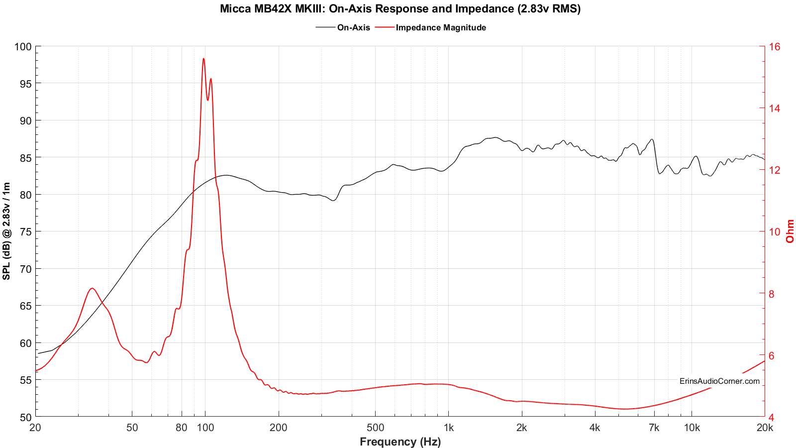
Frequency Response:
Notes about measurements (click for info)
Frequency response data (horizontal, vertical, “Spinorama”, polar, spectrograms, etc.) are all based on a 2.83 volts RMS logarithmic sweep at 1 meter to meet the standard sensitivity measurement spec. These data are captured using Klippel’s TRF module and a mixture of ground-plane measurement and 4-pi free-field measurement. Klippel’s In-Situ Room Compensation (ISC) module is then used with the ground plane measurement to provide a ‘reference’ curve to the 4-pi measurement which then corrects for the room’s influence and allows me to generate a reflection-free far-field response from an indoors measurement. Note: This is not a standard merge of nearfield and farfield nor a merge of ground-plane and farfield. Typical merged responses still suffer low resolution in the midrange where the response is merged due to the necessity of windowing the impulse response to remove reflections. One major downside to “gating” or “windowing” the impulse response is this low-resolution does not show resonance in the midrange. For example, most free-field measurements are only reflection-free until approximately 3 milliseconds, or about 300Hz. That means a data point every 300Hz. If you have a high-Q resonance at 450Hz the 300Hz resolution data will not show this resonance because the frequency resolution only has a data point at 300Hz and 600Hz; skipping right over the 450Hz. You would need a resolution of at least a half the width of the Q-factor; generally, 20Hz is adequate. However, 20Hz resolution is roughly 50ms of window-free response. The only way to achieve this is in a large parking lot or open field. Ground plane measurements are perfect for this but are subject to aiming/ground absorption (grass) and related issues above 400Hz. The ISC module permits results with as-close-to-anechoic as one can achieve without being anechoic. Thanks to the ISC module, the data I am providing here is higher resolution (~30Hz resolution) than an average person can provide without access to an anechoic chamber or the like.
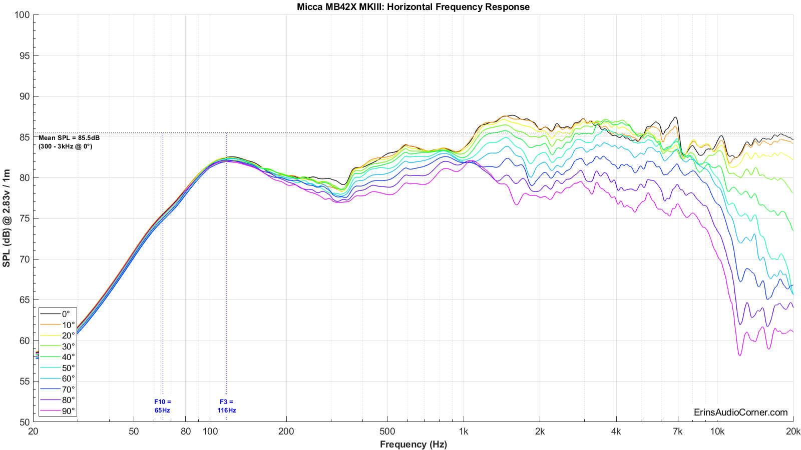
The measurement below provides the frequency response at the reference measurement axis - also known as the 0-degree axis or “on axis” plane - in this measurement condition was situated at the ribbon.
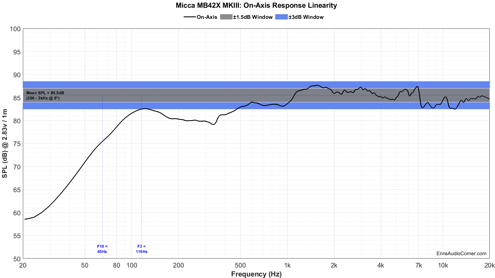
The mean SPL, approximately 85.5dB at 2.83v/1m, is calculated over the frequency range of 300Hz to 3,000Hz. But below about 1kHz it strays vastly from that mean and gets as low as 80dB at 300Hz.
The blue shaded area represents the ±3dB response window from my calculated mean SPL value. As you can see in the blue window above, the Micca MB42X Mark III is all over the place. There is nearly 5dB difference between the midrange and the treble.
The speaker’s F3 point (the frequency at which the response has fallen 3dB relative to the mean SPL) is 116Hz and the F10 (the frequency at which the response has fallen by 10dB relative to the mean SPL) is 65Hz.
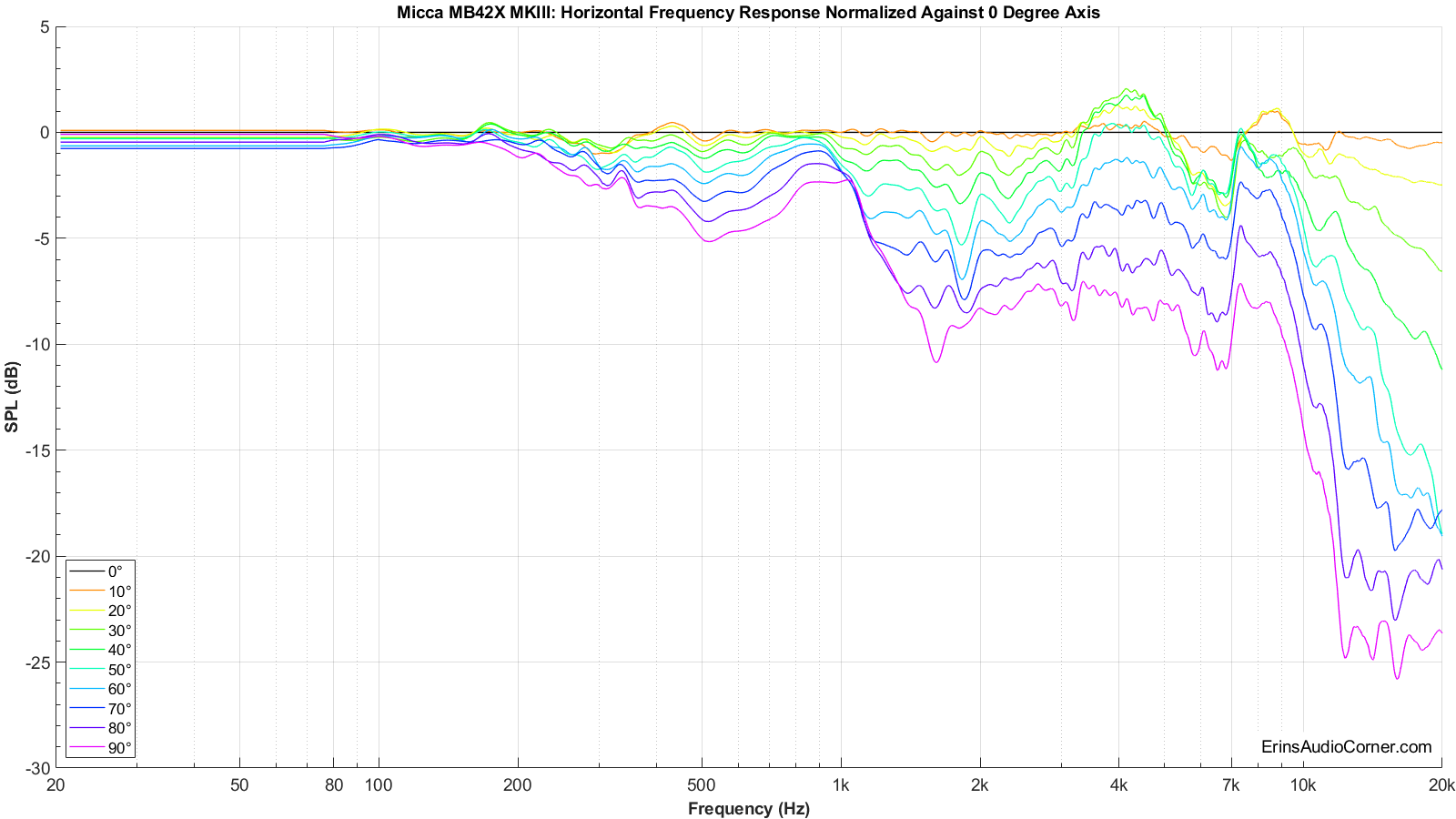
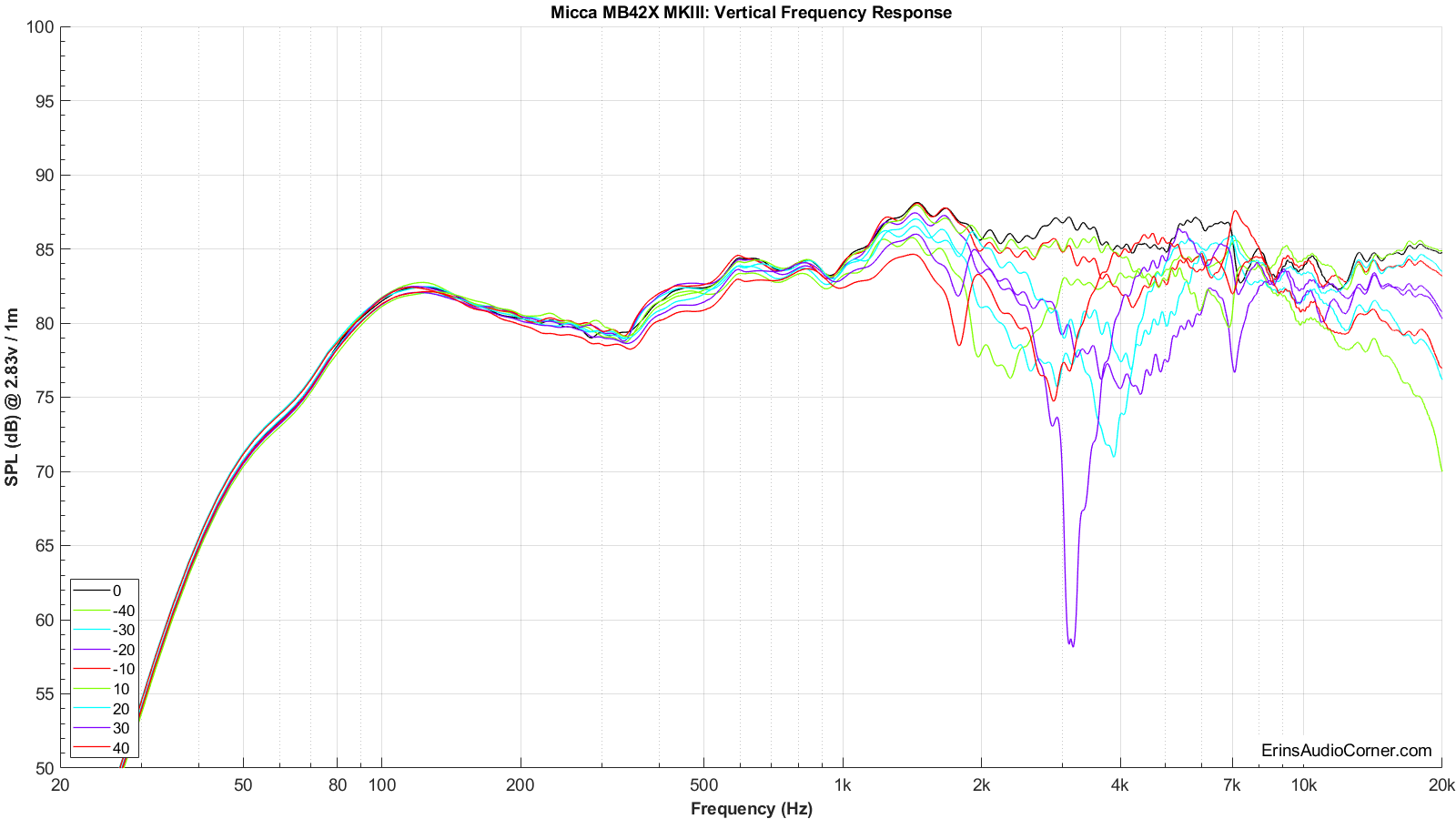
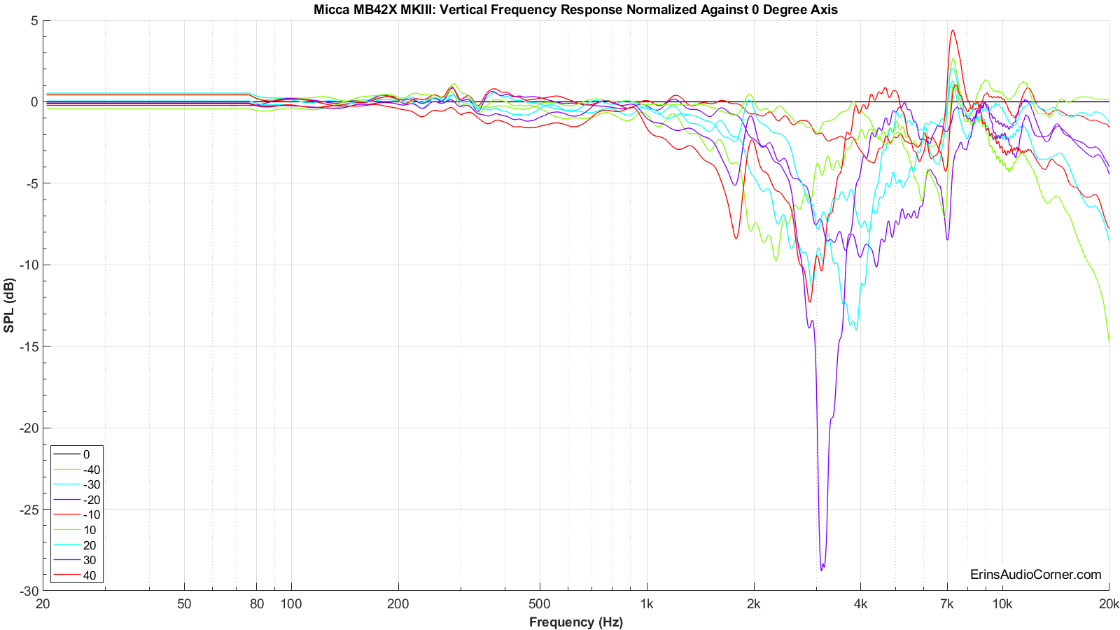
Below are both the horizontal and vertical response over a limited window (90° horizontal, ±40° vertical). I have provided a “normalized” set of data as well. The normalization simply means that I took the difference of the on-axis response and compared the other axes’ measurements to the on-axis response which gives the viewer a good idea of the speaker performance, relative to the on-axis response, as you move off-axis.
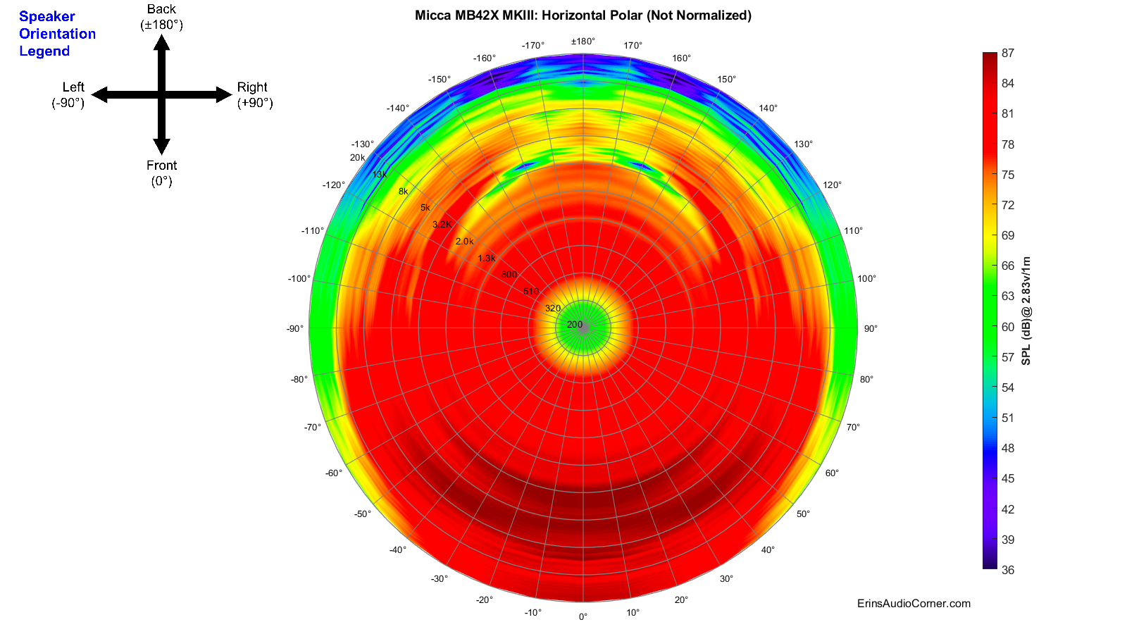
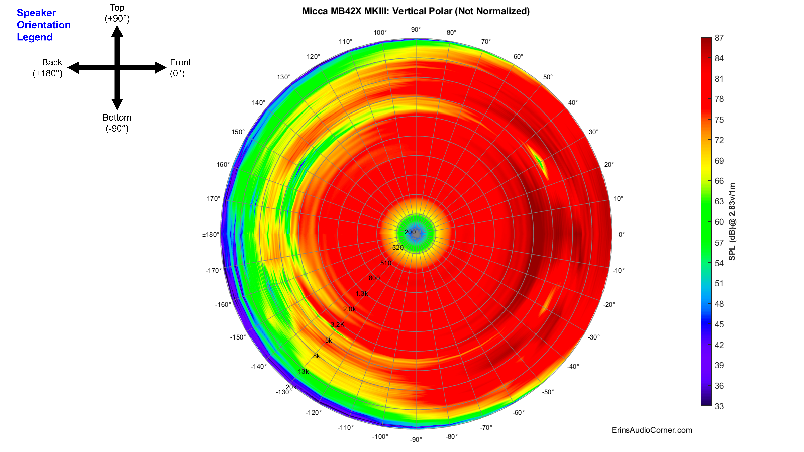
As I said above, the provided frequency response graphs were given with a limited set of data. I measured the response of the speaker’s vertical and horizontal axis in 10-degree steps over 360-degrees. Nearly 70 measurements in total are represented in my data. As you can imagine, providing all those data points in a single FR-type graphic below is a bit overwhelming and confusing for the viewer. A spectrogram is an alternate way to view this full set of data. This takes a 360-degree set of data and “collapses” it down to a rectangular representation of the various angles’ SPL. I have provided two sets of data: one set for horizontal and one for vertical. Each set consists of 2 graphics:
- Full response (20Hz - 20kHz with the angles from 0° to ±180°) with absolute SPL values
- Full, “normalized” response (20Hz - 20kHz with the angles from 0° to ±180°) with SPL values relative to the 0-degree axis
Normalized plots make it easier to compare how the speaker’s off-axis response behaves relative to the on-axis response curve.
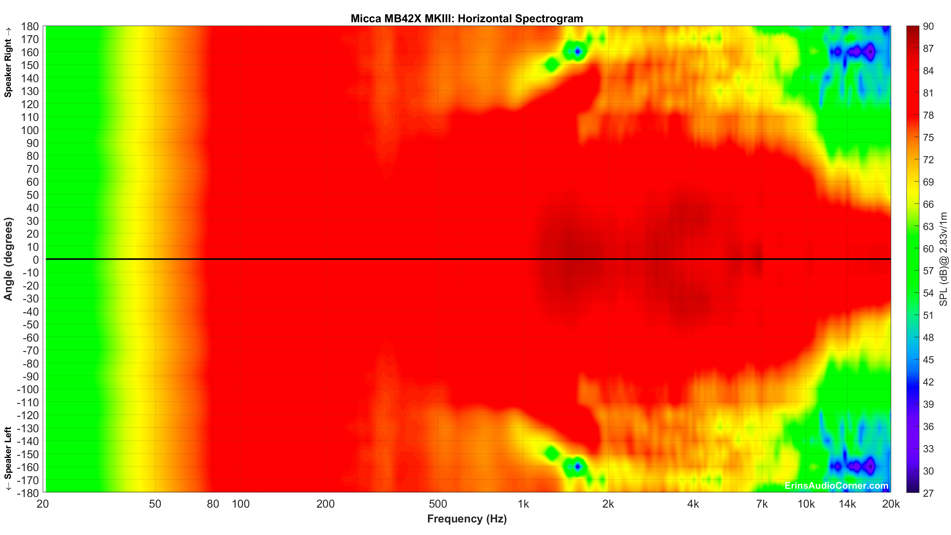
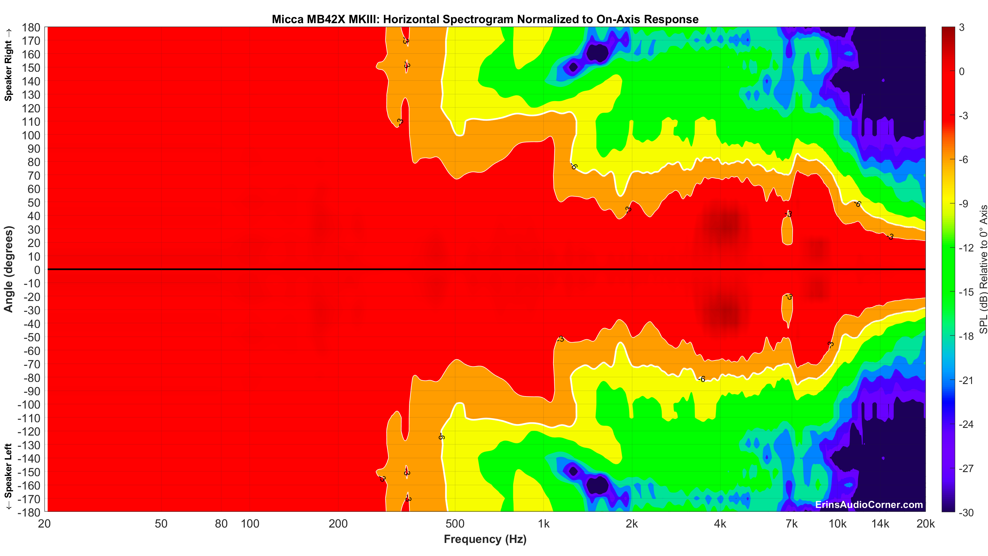
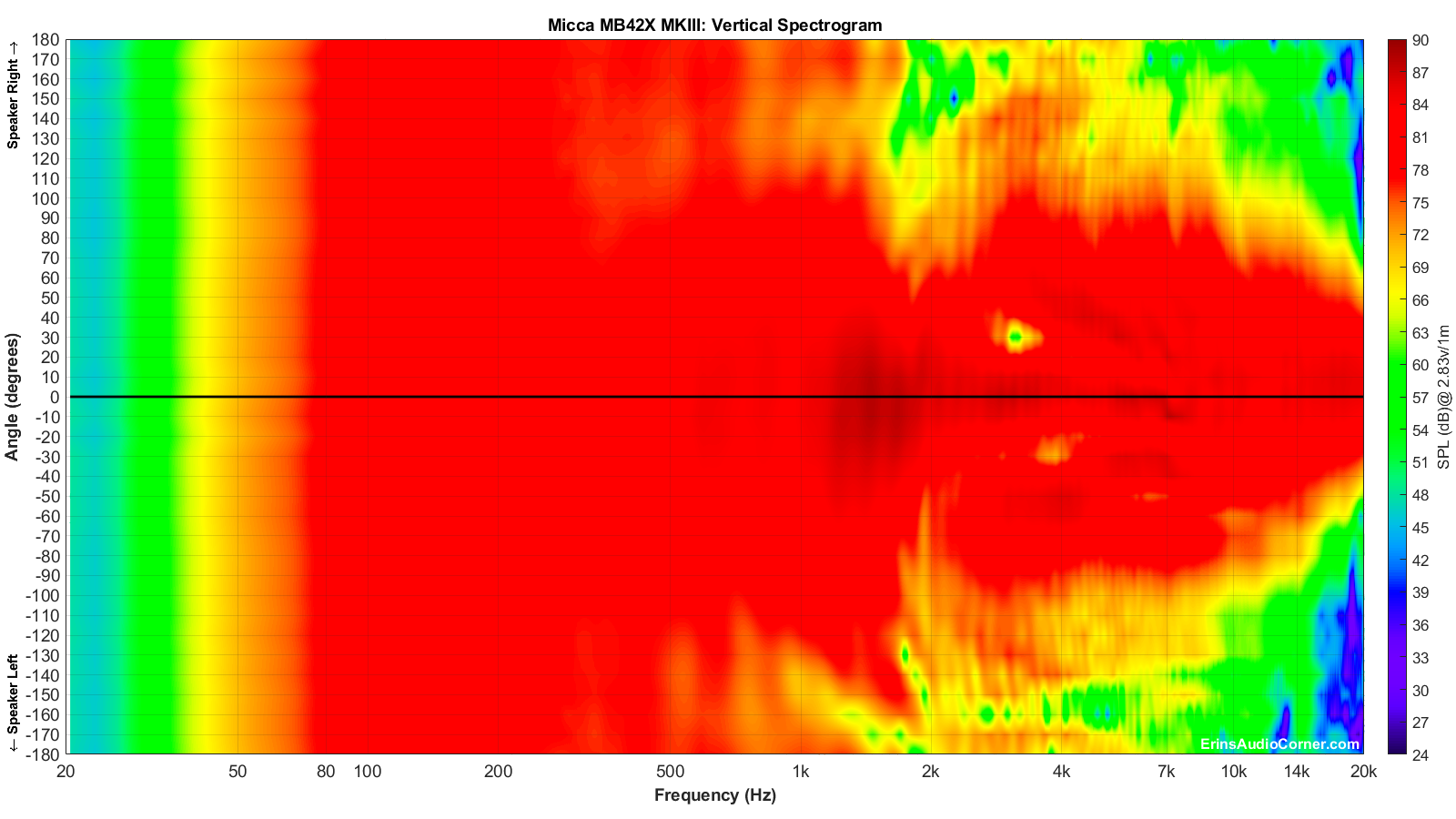
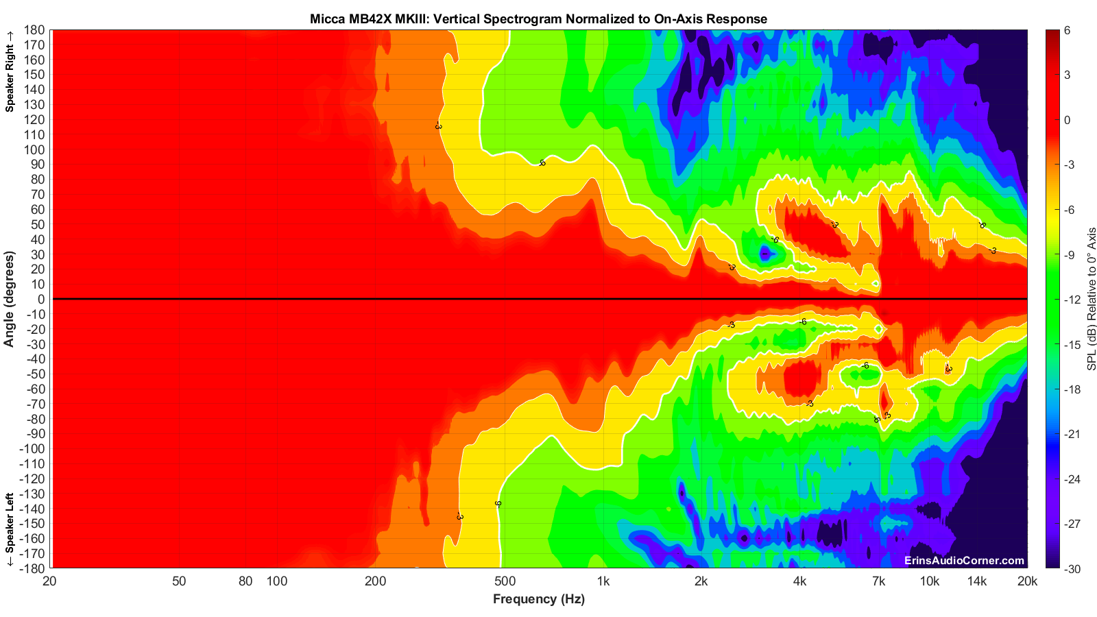
The above spectrograms are the standard way of providing directivity graphics by most reviewers. Some prefer not to normalize the data. Some prefer to normalize the data. Either way, it’s a useful visual to get an idea of the directivity characteristics of a speaker or driver.
However, these “collapsed” representations of the sound field are not very intuitively viewed. At least not to me. So, I came up with a different way to view the speaker’s horizontal and vertical sound field by providing it across a 360° range in a globe plot below. I have provided both an absolute SPL version as well as a normalized version of both the horizontal and vertical sound fields.
Note the legend provided in the top left of each image which helps you understand speaker orientation provided in my global plots below.
CEA-2034 (aka: Spinorama):
The following set of data is populated via 360-degree, 10° stepped, “spins” from vertical and horizontal planes resulting in 70 unique measurements. Thus, this is sometimes referred to as “Spinorama” data. Audioholics has a great writeup on what these data mean (link here) and there is no sense in me trying to re-invent the wheel so I will reference you to them for further discussion. However, I will explain these curves lightly and provide my own spin on what they mean (pun totally intended). Sausalito Audio also has a good write-up on these curves here. Furthermore, you can find discussion in Dr. Floyd Toole’s book “Sound Reproduction”. Here’s my Amazon affiliate link if you want to purchase it and help me earn about 2% of the price. And, finally, here is a great video of Dr. Toole discussing the use of measurements to quantify in-room performance.
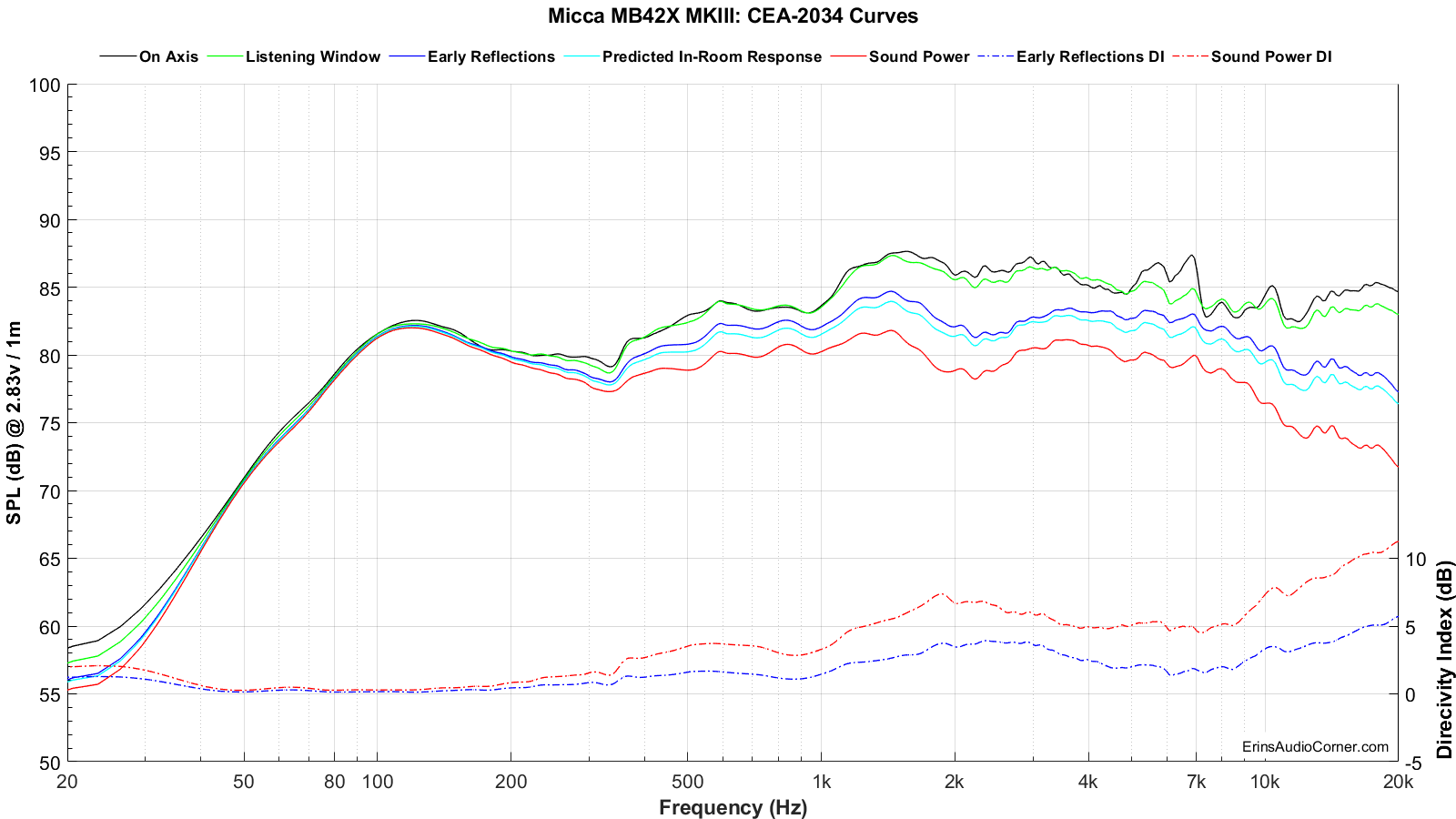
In short, the CEA-2034 graphic below takes all the response measurements (horizontal and vertical) and applies weighting and averaging to sub-sets and can help provide an (accurate) prediction of the response in a typical room. If there is a single set of data to use in your purchase decision, this is probably it.
Alternatively, click this arrow, if you want my quick take on what these curves mean without going to another site.
- On-Axis is simply the on-axis response. This is the 0-degree response curve.
- Listening Window is an average of the 0° to ±30° horizontal and 0° to ±10° vertical response curves and is used to understand what listeners typically hear in a home at the sweet spot, or Main Listening Position (MLP). The reason for this extended window of sound is simply because your room makeup might differ from another’s. This curve is an attempt to quantify a speaker’s performance over a smaller window that is often the norm for listening angle differences in various homes. It is important for this curve to very closely mimic the on-axis response. Deviations of the Listening Window curve relative to the on-axis response curve indicates a compromise in the speaker; often caused by directivity changes (as a speaker transitions from one drive-unit to another a la midwoofer to tweeter, or as a tweeter’s response becomes highly directional).
- Early Reflections is very useful because it helps us determine how the room’s influence will alter (corrupt, most of the time) the direct (on-axis) response. Ideally, the speaker radiates sound uniformly with no aberrations; no resonance, no directivity changes as the speaker transitions from the mid to the tweeter and so on. Because speakers often have these issues, however, what is reflected to us from the walls, ceiling and floor is not the same as what we hear from the on-axis, direct sound. And that’s a problem. Why is that a problem? As stated in Dr. Toole’s book “these are very influential in establishing timbral and spatial qualities”. Large deviations in this relative to the on-axis response also indicate areas where the room is of consequence. Also, it is important to understand the Early Reflections response is made up of rear-firing sounds. A speaker drive-unit is omnidirectional (radiating in all angles evenly) until the half-wavelength equals that of the drive-unit diameter. When the diameter is larger than the wavelength being played, the sound transitions from omnidirectional to directional; also known as “beaming”. Even tweeters beam. For example, a 1-inch dome tweeter will beam at approximately 6750Hz (speed of sound ÷ 2 ÷ diameter). In most speakers you have a single tweeter, firing forward. You can imagine that the high-frequency response in the front of the speaker would therefore be quite different than what is measured behind the speaker. So, being that the Early Reflections curve includes rear-hemisphere measurements you can understand that the high-frequency response would slope downward vs the on-axis response. This is understood and accepted.
- Predicted In-Room Response curve has the benefit of showing directivity mismatches at the crossover as well as resonances easily by comparing them to the overlaid Target curve (further down).
- Directivity Index (DI) curves are the difference in the Listening Window and the respective Early Reflections or Sound Power curves. My understanding, currently, is the Sound Power and Sound Power DI aren’t quite as useful for typical homes. However, there is emphasis placed on the Early Reflections DI curve. The right Y-Axis provides a value associated with the DI curves. The higher the number, the more directional the speaker. For example: a “0” DI curve - a curve which is completely flat - would be a speaker that is purely omnidirectional; radiating uniformly in all angles vertically and horizontally. A speaker that increases over frequency means that it is radiating in a tighter window as you increase in frequency. This is typical because, as I discussed above, even tweeters beam… and most speakers have a single tweeter facing the front and therefore, the speaker becomes directional at whatever the tweeter’s beaming frequency is. There isn’t necessarily a one-size-fits-all DI curve value. Though, it seems people (myself included) prefer a speaker with a wider soundstage which is found in lower directivity speakers (because more sound is bouncing off the side walls; which confuses the use of side-wall absorption but that’s for a later debate). However, what is important is that the curve, however tall you may prefer it to be, is smooth; almost linear. Dips and peaks mean that something, not good, is going on. But a linear curve indicates excellent transition through crossover regions, no resonance, etc. Since speakers are not perfect, though, linear DI curves are not the norm. Speakers become directional as they increase in frequency, around strong resonances, and as the sound transitions at the crossover from one drive-unit to another and you wind up with areas with peaks and/or dips whether they’re spread through a wide frequency range (low-Q) or very sharp/drastic (high-Q). But when you’re looking at the Early Reflections DI curve, look for this: smooth.
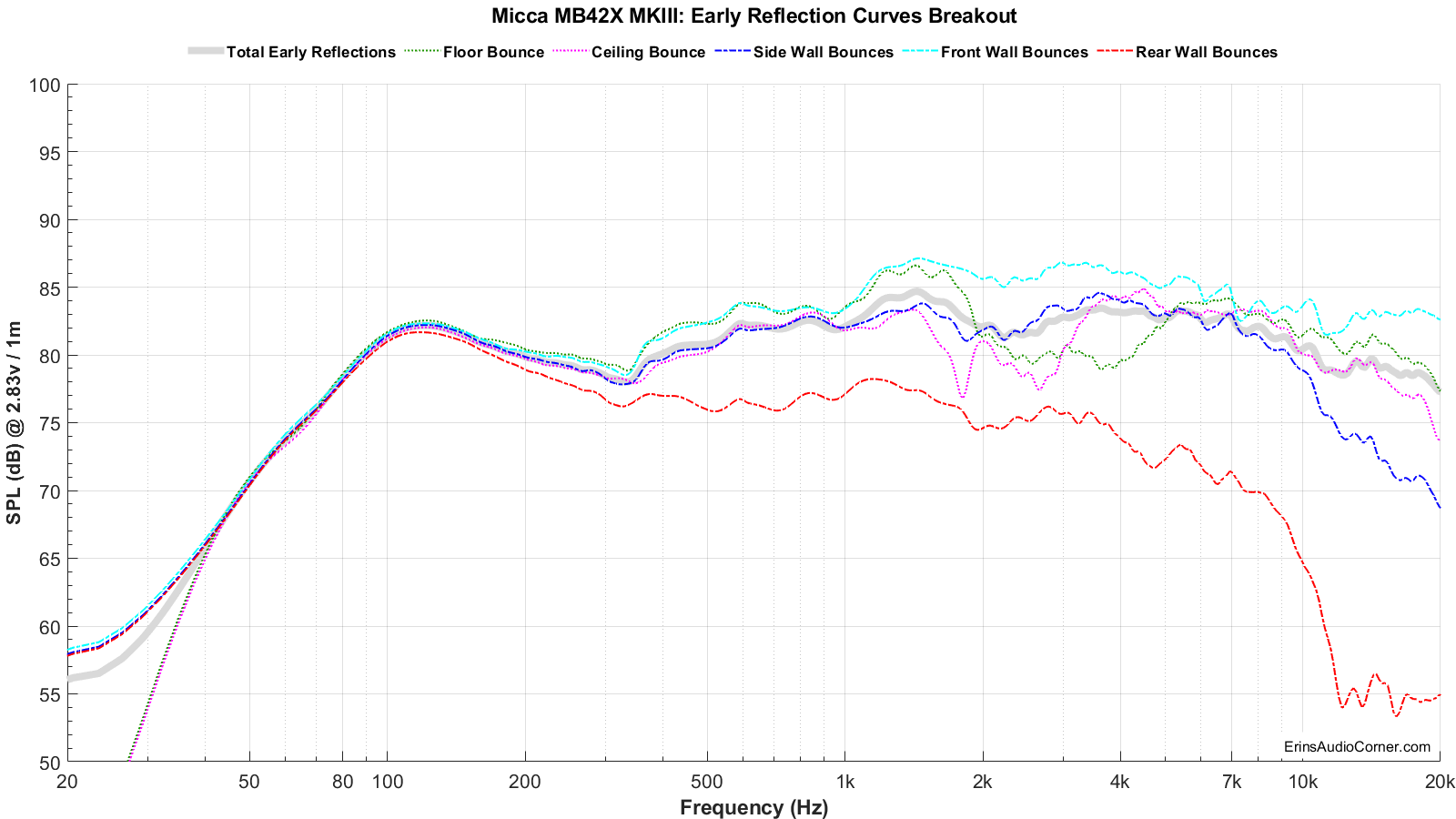
Below is a breakout of the typical room’s Early Reflections contributors (floor bounce, ceiling, rear wall, front wall and side wall reflections). From this you can determine how much absorption you need and where to place it to help remedy strong dips from the reflection(s). Again, as a pointer to the wide horizontal envelope, notice how the Rear Wall Bounces Curve is relatively high in amplitude (for a front-facing tweeter, at least) until about 10kHz.
And below is the Predicted In-Room response compared to a general Target curve equaling -1dB/octave.
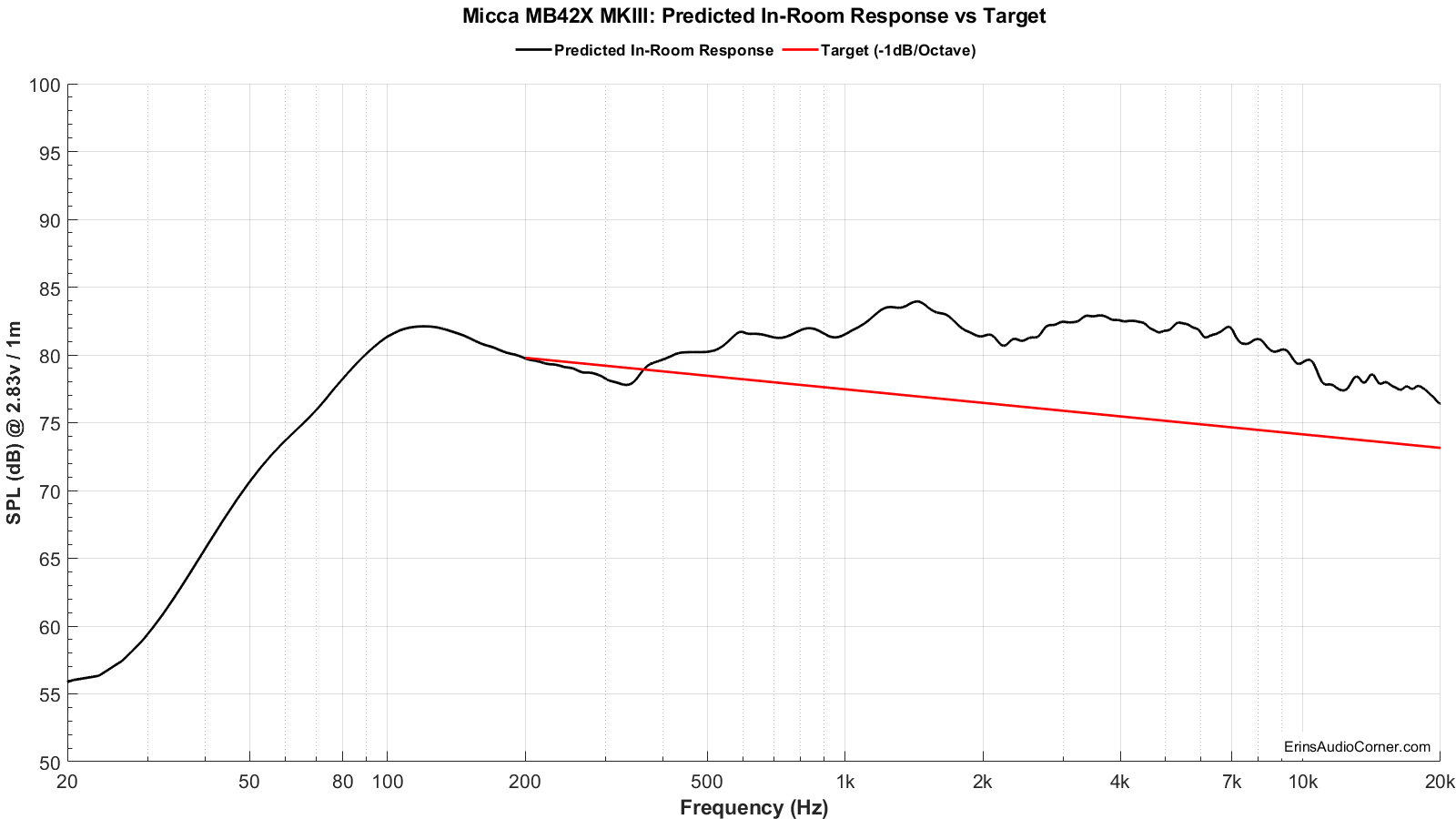
You may ask just how useful the above prediction is. Well, I’d be remiss for not delving in to that a little bit here. Please see my Analysis section below for discussion on this. :)
Total Harmonic Distortion (THD) and Compression:
Distortion and Compression measurements were completed in the nearfield (approximately 0.3 meters). However, SPL provided is relative to 1 meter distance.
Harmonic Distortion and Compression: What does this data mean? (click me for info)
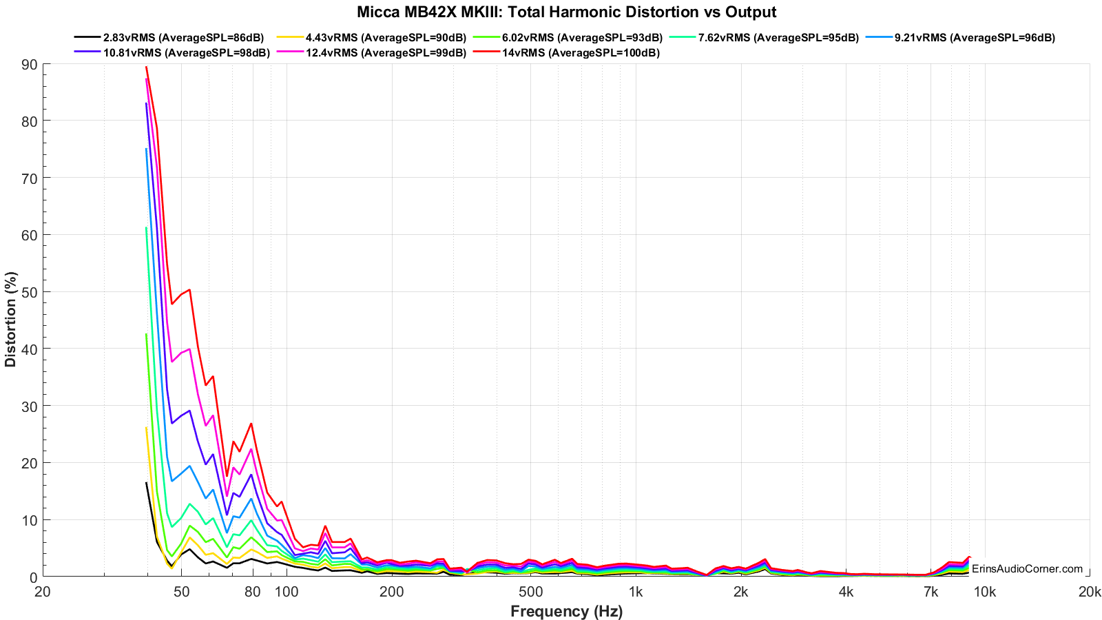
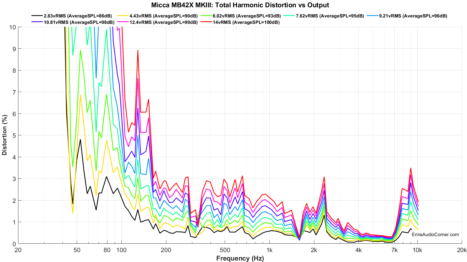
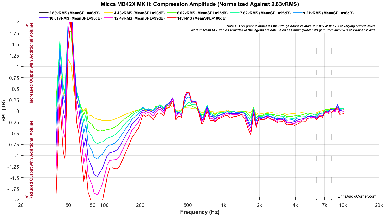
Harmonic Distortion and Compression are provided at varying levels to get an idea of what happens as the voltage into the speaker is increased and overall output volume increases. The “mean spl” values associated with each voltage provided in the legend is based on a calculation of expected volume assuming linear volume at the 300-3kHz region. Meaning, if a speaker is ideal and you tell your stereo to increase by 6dB by turning the volume knob +6dB, the output will increase by 6dB. In the real-world, however, a speaker is a mechanical device and there are compression effects that can limit the output volume and, therefore, you could possibly only get an actual increase in volume of 5dB. A good speaker will have little compression (< 1dB), where poorer speakers may suffer greater compression (> 2dB). Generally speaking, higher sensitivity speakers (like pro-audio speakers with 100dBSPL @ 2.83v/1m spec) suffer relatively no compression while lower sensitivity speakers (low 80’s dBSPL @ 2.83v/1m) suffer more compression. When a crossover is used the compression near the speaker’s Fs is attenuated and overall the compression effects are mitigated. With that in mind, what you see below is first the Total Harmonic Distortion at varying output levels.
Maximum Long Term SPL:
The below data provides the metrics for how Maximum Long Term SPL is determined. This measurement follows the IEC 60268-21 Long Term SPL protocol, per Klippel’s template, as such:
- Rated maximum sound pressure according IEC 60268-21 §18.4
- Using broadband multi-tone stimulus according §8.4
- Stimulus time = 60 s Excitation time + Preloops according §18.4.1
Each voltage test is 1 minute long (hence, the “Long Term” nomenclature).
The thresholds to determine the maximum SPL are:
- -20dB Distortion relative to the fundamental
- -3dB compression relative to the reference (1V) measurement
When the speaker has reached either or both of the above thresholds, the test is terminated and the SPL of the last test is the maximum SPL. In the below results I provide the summarized table as well as the data showing how/why this SPL was deemed to be the maximum.
This measurement is conducted twice:
- First with a 20Hz to 20kHz multitone signal
- Second with a limited 80Hz to 20kHz signal
The reason for the two measurements is because it is unfair to expect a small bookshelf speaker to extend low in frequency. Applying both will provide a good idea of the limitations if you were to want to run a speaker full range vs using one with a typical 80Hz HPF. And you will have a way to compare various speakers’ SPL limitations with each other. However, note: the 80Hz signal is a “brick wall” and does not emulate a typical 80Hz HPF slope of 24dB/octave. But… it’s close enough.
You can watch a demonstration of this testing via my YouTube channel: https://youtu.be/iCjJufvW0IA
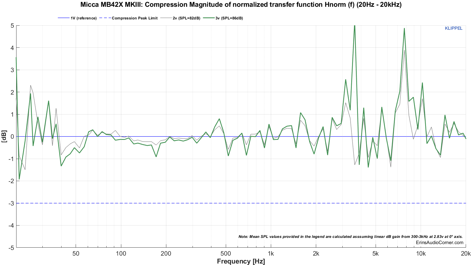
Test 1: 20Hz to 20kHz
Multitone compression testing. The red line shows the final measurement where either distortion and/or compression failed. The voltage just before this is used to help determine the maximum SPL.
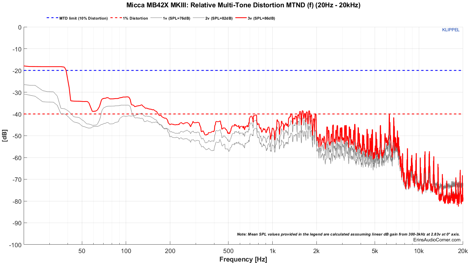
Multitone distortion testing. The dashed blue line represents the -20dB (10% distortion) threshold for failure. The dashed red line is for reference and shows the 1% distortion mark (but has no bearing on pass/fail). The green line shows the final measurement where either distortion and/or compression failed. The voltage just before this is used to help determine the maximum SPL.
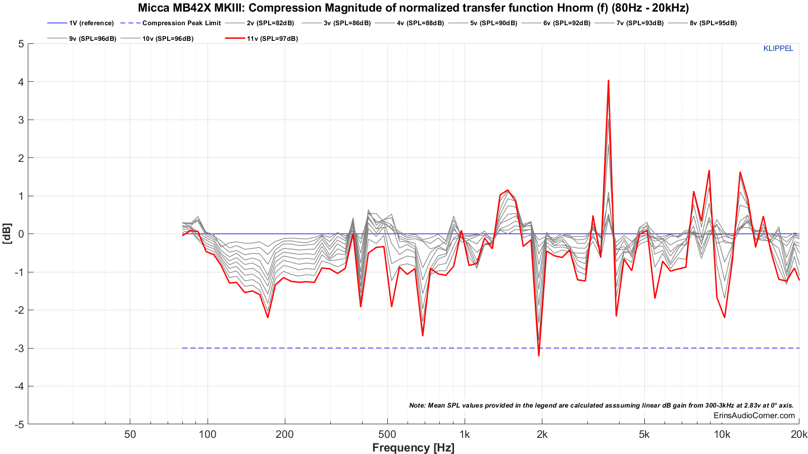
Test 2: 80Hz to 20kHz
Multitone compression testing. The red line shows the final measurement where either distortion and/or compression failed. The voltage just before this is used to help determine the maximum SPL.
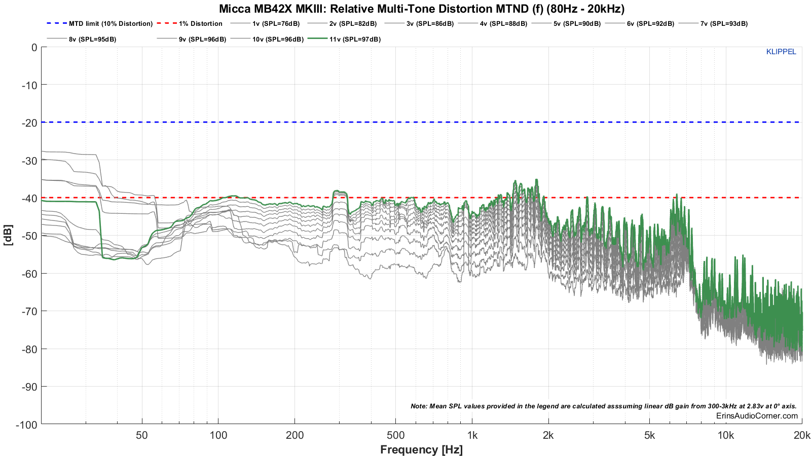
Multitone distortion testing. The dashed blue line represents the -20dB (10% distortion) threshold for failure. The dashed red line is for reference and shows the 1% distortion mark (but has no bearing on pass/fail). The green line shows the final measurement where either distortion and/or compression failed. The voltage just before this is used to help determine the maximum SPL.
The above data can be summed up by looking at the tables above but is provided here again:
- Max SPL for 20Hz to 20kHz is approximately 88dB @ 1 meter. The distortion threshold was exceeded above this SPL.
- Max SPL for 80Hz to 20kHz is approximately 100dB @ 1 meter. The compression threshold was exceeded above this SPL.
Extra Measurements:
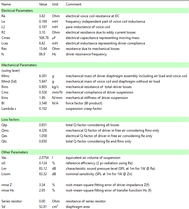
Thiele-Small and Large Signal Analysis: Using Klippel’s Distortion Analyzer 2, Linear Lumped Parameter Measurement Module, Pro Driver Stand and provided Panasonic ANR12821 Laser along with Klippel’s Training 1 - Linear Lumped Parameter Measurement tutorial, I measured this drive unit’s impedance and small-signal parameters. Below are the results.
The few standouts to me are:
- High Fs of ~87Hz
- High Qts of ~0.850
- Low Sensitivity of ~ 83dB
All of these parameters translate to a speaker that needs to large enclosure (so the Qtc will not be any larger; as the Qts itself is already relatively high), high low cutoff point (due to high Fs) and low sensitivity (even though the on-axis average SPL is ~ 85.5dB, the SPL in the bass region is in the low 80’s).
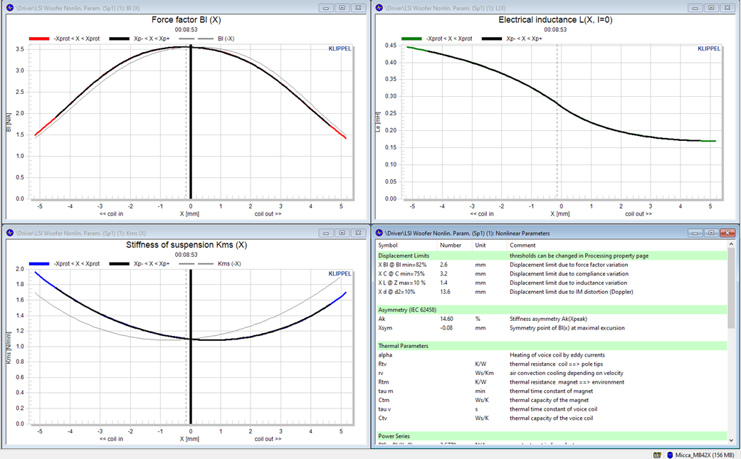
Using Klippel’s Distortion Analyzer 2, Large Signal Identification Module, Pro Driver Stand and provided Panasonic ANR12821 Laser along with Klippel’s Training 3 - Loudspeaker Nonlinearities tutorial, I measured the linear, nonlinear and thermal parameters of this drive unit. Below are the nonlinear results.
The linear excursion is capped at 1.4mm one-way due to inductance variation. It’s rare I have a mid/woofer be limited in excursion due to inductance. And in a speaker like this; one that is most likely to be used from 80Hz all the way out to 20kHz, that is a problem. This result indicates the mid/woofer will have a very high level of mid-to-upper frequency distortion if the cone is asked to play content near Fs due to high inductance. And with a bookshelf speaker like this, it should absolutely be crossed above 100Hz to limit any playback near the Fs of 87Hz.
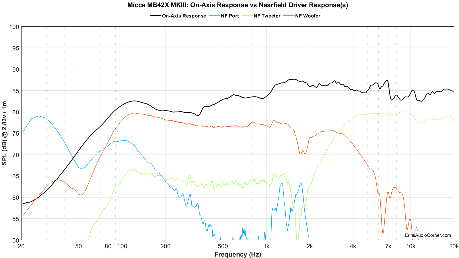
Nearfield measurements.
Mic placed about 0.50 inches - relative to the baffle - from each drive unit and port. While I tried to make these as accurate in SPL as I could, I cannot guarantee the relative levels are absolutely correct so I caution you to use this data as a guide but not representative of actual levels (measuring in the nearfield makes this hard as a couple millimeters’ difference between measurements can alter the SPL level).
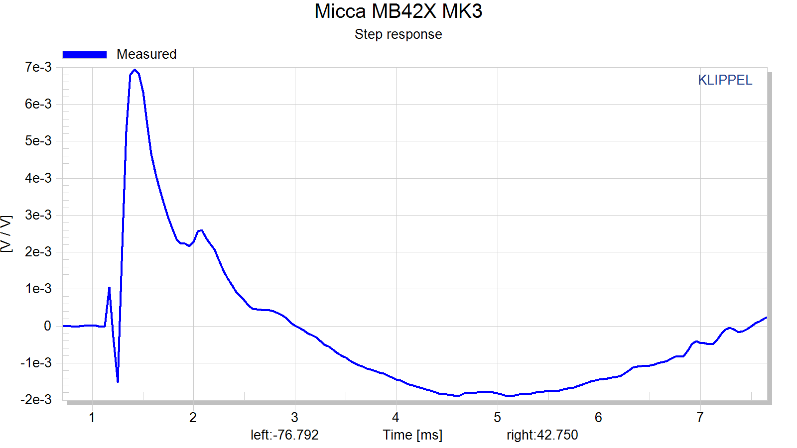
Step-Response.
Subjective Evaluation:
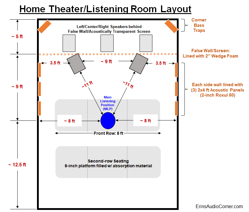
Before I dive in to the subjective feedback let me first give you the layout of my room…
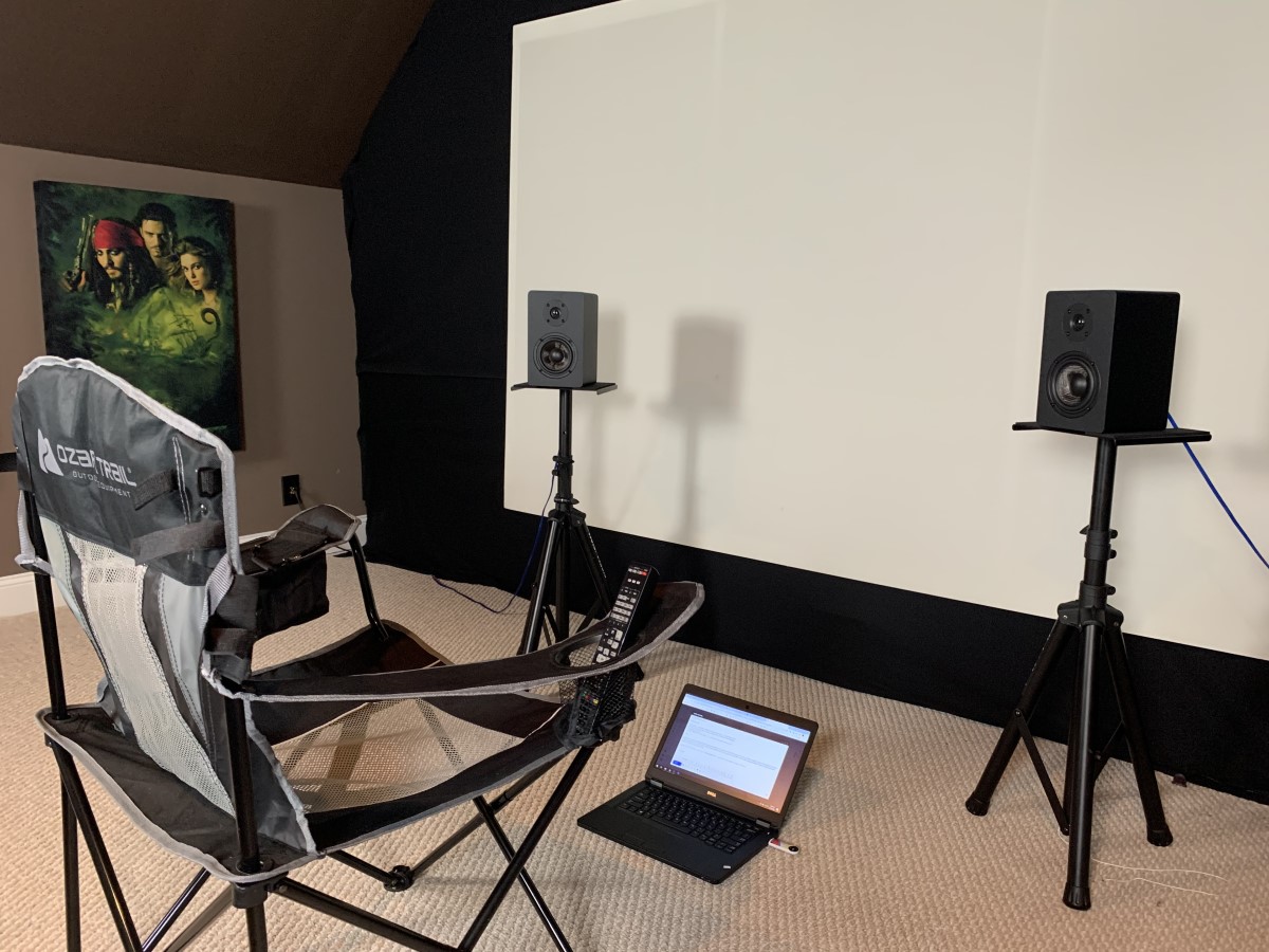
And here is the nearfield setup (with the lawn chair in all its glory).
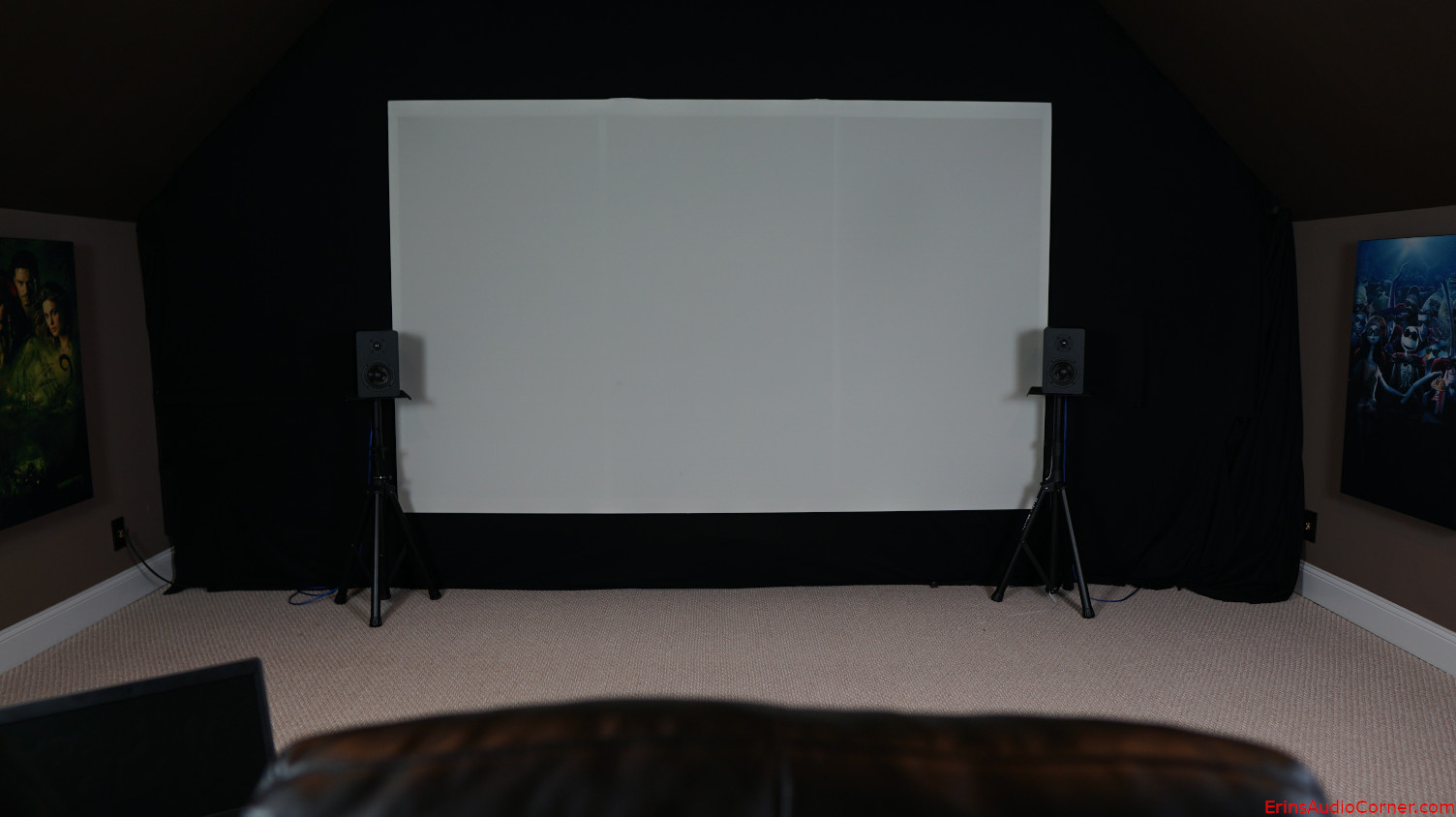
I don't like seeing speakers when watching a movie. So, I built a false wall and used an acoustically transparent screen with speakers behind it. The wall is only 2x4's; no panels of wood or anything. Just a skeleton of a wall to give me something to attach the screen and acoustic treatment to. There is 2-inch wedge foam affixed to the 2x4 studs and between the false wall and back of the room are the front speakers (L/C/R & 18-inch subwoofers).
My demo music:
| Title | Artist | Album |
|---|---|---|
| Enjoy The Silence | Depeche Mode | Best Of Depeche Mode, Vol. 1 |
| Higher Love | Steve Winwood | Back In The High Life (MFSL UDCD-611) |
| 24K Magic | Bruno Mars | 24K Magic |
| Magic | The Cars | Heartbeat City (MFSL) |
| Everlasting Love | Howard Jones | The Best of Howard Jones |
| Kodachrome | Paul Simon | There Goes Rhymin’ Simon |
| Everybody Wants To Rule The World | Tears for Fears | Songs from the Big Chair (2014 Deluxe Edition - Disc 1) |
| Know Your Enemy | Rage Against The Machine | Rage Against The Machine (Hybrid SACD) |
| Doo Wop (That Thing) | Lauryn Hill | The Miseducation of Lauryn Hill |
| Tell Yer Mama | Norah Jones | The Fall |
| Don’t Save Me | HAIM | Days Are Gone |
| He Mele No Lilo | Mark Keali’i Ho’omalu and Kamehameha Schools Children’s Chorus | Lilo And Stitch |
| Wrapped Around Your Finger | The Police | Synchronicity |
| Sledgehammer | Peter Gabriel | So |
| Feel It Still | Portugal. The Man | Woodstock |
| Free Fallin | John Mayer | Where The Light Is |
| Whiplash | The Swampers | Muscle Shoals Has Got The Swampers |
Note: I don’t generally audition speakers with the typical “audiophile” music. I have thousands of high-quality albums ranging from pop to metal to jazz and all around. I don’t typically listen to “audiophile” music because I just don’t enjoy it. It is far more important that your evaluation music be something you are familiar with than it is to be esoteric for the sake of being esoteric. You also want to listen to music you enjoy because auditioning a stereo system shouldn’t feel like a chore. Such is the case in my evaluations. Besides, the subjective evaluation is purely to help tie to the objective data and make sense of what I am hearing to help you all get an understanding of how relevant the data is. As you will see below, my music selection did a great job at providing enough range for me to identify the issues that readily appear in the data.
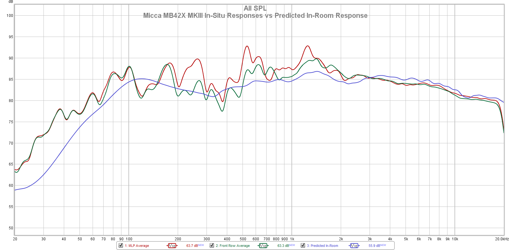
Let’s look at the measured in-room response I captured using my UMIK-1 and REW. Notice how well it matches the predicted in-room response.
- Red = MLP Average (average response in the head area at the main listening position)
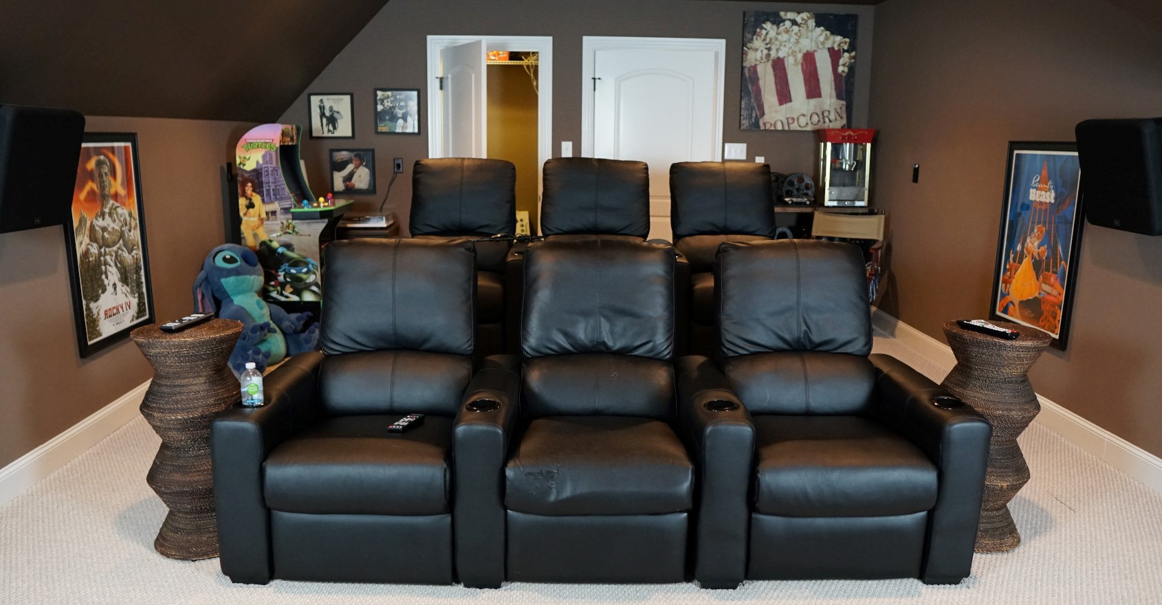
- Green = Front Row Average (average across front 3 seats in my home theater)
- Blue = Predicted In-Room Response from the data
Subjective Analysis Setup:
- The speaker was aimed on-axis with the vertical listening axis between the mid and tweeter per Micca’s manual (which states to place the speaker on a stand with the stand height 6-inches below your ear; putting the ear height between the mid and tweeter).
- I listened first at my typical listening position about 11 feet away. I then moved to the nearfield, roughly 3 feet from the speakers.
- I used Room EQ Wizard (REW) and my calibrated MiniDSP UMIK-1 to get the volume on my AVR relative to what the actual measured SPL was in the MLP (~11 feet from the speakers). I varied it between 85-90dB, occasionally going up to the mid 90’s to see what the output capability was. In a poll I found most listen to music in this range.
- All speakers are provided a relatively high level of Pseudo Pink-Noise for a day or two - with breaks in between - in order to satisfy any “break-in” concerns.
- I demoed these speakers without a crossover and without EQ.
- Components: Oppo BDP-103 playing music off my thumb drive feeding signal via HDMI to a Denon AVR-X4000 which then feeds in to a refurbished Adcom GFA-545 for power.
I listened to these speakers and made my subjective notes before I started measuring objectively. I did not want my knowledge of the measurements to influence my subjective opinion. This is important because I want to try to correlate the objective data with what I hear in my listening space in order to determine the validity of the measurement process. I try to do a few listening sessions over a couple days so I can give my ears a break and come back “fresh”.
Here’s the rundown of my subjective notes and where it fits with objective:
- Overall, I found the max SPL I could drive the speakers to was around 88-90dB at my listening position, depending on the music. In the nearfield listening, the output was about the same level because of distortion limitations; I didn’t like them above 90dB.
- Depeche Mode’s “Enjoy The Silence”: sounds distant; hollow through the entire midrange. No bass below ~160hz. Well, looking at the data we see a big trough smack in the midrange at about 300Hz. The treble is also about 5dB higher than the midrange.
- Steve Winwood’s “Higher Love”: Wide left soundstage; missing something below 1kHz tonally; hollow sounding. Not “involving”. Just “there”.
- Bruno Mars’ “24K Magic”: Biting highs somewhere above 4kHz. Midbass was lacking emphasis.
Overall?…. YUCK. At this point I decided to move closer to see if listening in the nearfield would help (spoiler: it didn’t).
- The Police “Wrapped Around Your Finger”: There’s nothing in the bassline below about 140Hz.
- Portugal The Man’s “Feel It Still”: The only song that had a positive attribute which was around about 800Hz which sounded the most natural so far. Looking back at the data, this is the only area in the response that is linear within about 1/2-Octave above/below.
- Norah Jones “Tell Yer Mama”: Mechanical noise… Tinsel lead slap? Note, again, the volume wasn’t that loud.
… and that’s it. I made it through about 7 songs before I just stopped. I couldn’t take listening to the speakers anymore. They were that bad.
I chose not to run Dirac Live with these speakers because I wouldn’t recommend anyone buy these and I didn’t want to waste my time with these speakers anymore.
Bottom Line
The Micca MB42x MKIII is a terrible speaker if you intend to listen to it as a budget audiophile speaker (or anything resembling that). There. I said it.
Micca lists these “Feature Highlights” on their site:
- Balanced woven carbon fiber woofer for enhanced transient and impactful bass
- High performance silk dome tweeter for smooth treble and accurate imaging
- Highly optimized 9-element crossover with full 18dB/octave* alignment and compensation network
- Ported enclosure delivers extended bass response with low distortion
- Dramatically transformed sound signature that is incredibly open, balanced, and dynamic
That’s a big “no” to every-single-one of the above “features”.
It suffers extreme non-linearity and high distortion. While I think anyone in their right mind would know not to expect tons of output (not just bass; but overall volume) from a speaker this size, what you would expect is a semblance of linear frequency response. This speaker does not have that at all. The midrange exhibits a trough centered on ~300Hz. The difference in the midrange to upper-midrange/low-treble is nearly 5dB and then a 3dB dip from low-treble to upper-treble above 7kHz. This results in a very “hollow” sound in the midrange and rather “forward” sounding presence region followed by a lack of upper end detail and sense of space (also thanks to the increasing directivity of the tweeter).
As for bass… well, there’s really not much there. But, again, it’s a small bookshelf speaker with a 4-inch mid. There is a high-Q peak centered around 115Hz but that doesn’t do much except add some unnatural ‘umph’ to kickdrums via the harmonic. But, again, since this region is down so low relative to the treble region, it doesn’t really help.
Placing these speakers near a wall would help the midrange out but in doing so you just boost the overall response; meaning you also boost the trough in the midrange and the high-Q midbass bump. Plus, the rear port would be blocked killing the low end contribution it provides. Meaning that placing the speaker against a wall would be pointless.
Distortion is very high below 200Hz with greater than 5% THD at typical listening levels. Above this, the distortion is anywhere from 2-3% THD in the midrange at these same listening levels.
Unless you absolutely need a speaker this size, you have the ability EQ until your heart (or ears) is content and you don’t plan on listening louder than talking levels in the nearfield… don’t buy this speaker. Buy the Neumi BS5 if you’re looking for a budget set of bookshelf speakers. That’s an easy, easy decision. Comparatively, this Micca speaker isn’t even in the same ballpark. It’s not even worthy enough to hold a baseball. Here’s the Neumi via my Amazon link again, if you want to buy them through my affiliate link and help the site out:
Contribute
If you like what you see here and want to help me keep it going, you can donate via the PayPal Contribute button at the bottom of each page. If you can help by chipping in, I would truly appreciate it.
You can also join my Facebook and YouTube pages if you’d like to follow along with updates.
Thanks!